Introduction
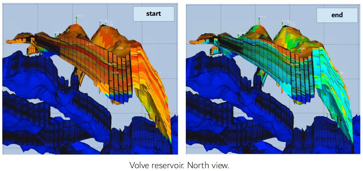
Continuing with the previous article The fabrication of an artificial intelligence agent for reservoir history matching from the Volve dataset, and the generation of a master dataset for an AI agent to perform history matching of reservoir models, we will extract additional data from the output of the Volve reservoir model, the PRT text file. This is the output “as-is”, as we found it. No additional simulation runs have been performed over this model.
In addition to the PRT file there are binary files that Eclipse generates as part of the output. We still don’t have a reader for those files but we are close to take a look at some code written in Python by a Reservoir Engineer who I have been in touch for the past few days. Working with binary files should be your more preferred option than dealing with the painful extraction of variables using regular expressions (regex). At any rate, we could take these last two posts as an exercise of applying regex to text files when we don’t have access to the binary files format.
Data blocks in the simulator output
In the previous article, we extracted the field totals, or cumulatives, from the text blocks with the keyword BALANCE AT in the PRT file; produced volumes of oil, gas and water as well as the COIP, or currently oil in place. There is another block of interest in the text file, that we could call the STEP block. This block contains instantaneous production variables such as GOR, watercut, WGR and the average bottomhole pressure (PAV). WHat we are looking here is to improve the current dataset from containing cumulative volumes to include these new production variables. In other other words, we want a more comprehensive dataset that we could use as part of a machine learning algorithm later.
Challenges ahead
There are some challenges though while doing this:
The number of observations (rows) of the variables extracted from the STEP block is greater than the observations of the field totals dataset.
Since the data originated from the STEP block is more granular than that of the BALANCE-AT block, we will face the challenge of mismatched dates between both. So, a more complete dataset of production variables comes with its costs. Merging two dataframes will have to be carefully performed and inspected.
Additionally, we may not getting all the variables from the PRT text file as from the binary files generated by Eclipse. As one of the reservoir engineers, who read the previous article, noticed there is an inconsistency in the produced water between the PRT file values I got and the binary files he was able to read using his code. This is one of the drawbacks of reading the PRT text file and mining for data; it is difficult to find all the output variables from the simulation, and some of them -if not properly identified- could be misleading. Also, how remarkable is seeing reproducibility at work! A colleague was able to detect an error in my data extraction.
While the extraction of data from a text file serves a purpose, when a reader of binary files from the simulation is not available, we should exercise caution with those extracted values from a text file.
It is nice to get a good match of volumes between simulation and the real world. But we also have to be prepared for the bad news: when one of the reservoir fluids is far, far away from the match.
Read the simulation output data
Read the PRT text file
As we did in the previous step, we start by reading the reservoir simulation output file: the text file VOLVE_2016.PRT`. It is a relatively big file: 228 megabytes. I have zipped it in order to save some disk space and prevent Github from complaining about the size of the file. Maximum size of a file in Github is 100 megabytes.
This data operation was shown in the previous article with the only difference that I used Google drive instead. In a second case, I used Zenodo, a service that allows sharing datasets up to 50 gigabytes per dataset. I am providing the links to the datasets living in Zenodo at the end of this article.
library(dplyr)
library(ggplot2)

# read the Eclipse PRT output report
# proj_root <- rprojroot::find_rstudio_root_file()
proj_root <- "./"
# had to zip the PRT file because it's 225 MB and too big for Github
volve_2016_zip <- file.path(proj_root, "inst/rawdata", "VOLVE_2016.zip")
temp <- tempdir()

volve_2016_txt <- readLines(unzip(volve_2016_zip, exdir = temp))
Once with the contents of VOLVE_2016.PRT loaded in the object volve_2016_txt, we proceed to perform the extraction.
We start by extracting few rows after the STEP keyword.
# get a list of rows from " STEP"

# find the rows where we find the word " STEP"
step_rows <- grep("^ STEP", volve_2016_txt)

# add rows ahead to where the keyword was found
step_info_range <- lapply(seq_along(step_rows), function(x)
    c(step_rows[x], step_rows[x]+1:2))               # add two extra row indices

step_info_range[[1]]   # sample for report page 1 only
#> [1] 1548178 1548179 1548180
These extra row indices are lines of text where the report keeps more information of the evolution of the simulation. Here is a couple of screenhots.
Step at day 1:

Figure 1: Step at 1 day
Step at day 3,197:
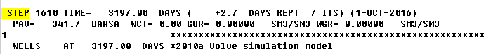
Figure 2: Step at 3197 days
Now, knowing the row indices for the text we need to extract from the PRT file, we can proceed to extracting those lines of text and putting them in a list, one page or one step, per list element. We do this to later iterate through all the steps and extract the data we want. The object steps_info_txt_pages is a list containing the row indices that are of our interest.
# get the text from all pages and put them in a list
steps_info_txt_pages <- lapply(seq_along(step_info_range), function(x)
    volve_2016_txt[step_info_range[[x]]])
For example, this is an example of the first page for step #1.
steps_info_txt_pages[1]
#> [[1]]
#> [1] " STEP    1 TIME=      1.00  DAYS (    +1.0  DAYS INIT  5 ITS) (1-JAN-2008)       "
#> [2] "  PAV=   329.6  BARSA  WCT= 0.00 GOR= 0.00000   SM3/SM3 WGR= 0.00000   SM3/SM3   "
#> [3] ""
Extracting step data from the text file
Extract the days from the STEP block
Although we could extract all the data we require from the text file in one go, it is better to see one or two examples of seeing regular expressions or regex at work. Regular expressions are practically available to all programming languages: C++, Java, JavaScript, Python, Perl, R, etc.
In this first example, we will extract the number of days at the current simulation step. If this is the first step page:
 STEP    1 TIME=      1.00  DAYS (    +1.0  DAYS INIT  5 ITS) (1-JAN-2008)
  PAV=   329.6  BARSA  WCT= 0.00 GOR= 0.00000   SM3/SM3 WGR= 0.00000   SM3/SM3
to extract the days we have to provide a regex pattern that detects a real number like 1.00, which is ".*?(\\d+.\\d.)+.*".
Explanation
.*?will match any characters. lazy matching.(\\d+.\\d.)capturing group.\\d+matches any number of digits\\d.matches a digit and then any character
Here we iterate through the list steps_info_txt_pages, extract the step-page, extract the number of days from the text. After that, we convert the vector to a dataframe.
# iterate through the list of STEP pages
days_dfs <- lapply(seq_along(steps_info_txt_pages), function(x) {
    page <- steps_info_txt_pages[[x]]   # put all pages text in a list
    days_row_txt <- page[1]                                # get 1st row of page
    days_value <- sub(".*?(\\d+.\\d.)+.*", "\\1", days_row_txt,
                      perl = TRUE) # extract the days

    # dataframe; days as double; no factors.
    data.frame(days = as.double(days_value), stringsAsFactors = FALSE)
})

days_df <- do.call("rbind", days_dfs)
Extract the days
Let’s see a sample of the first ten and last ten rows for the dataframe days_df just extracted:
rbind(head(days_df, 10), tail(days_df, 10))   # show the first 10 and last 10 rows
#>         days
#> 1       1.00
#> 2       1.63
#> 3       2.32
#> 4       3.50
#> 5       5.45
#> 6       8.22
#> 7      11.00
#> 8      14.61
#> 9      17.80
#> 10     21.00
#> 1601 1601.00
#> 1602 1602.00
#> 1603 1603.00
#> 1604 1604.00
#> 1605 1605.00
#> 1606 1606.00
#> 1607 1607.00
#> 1608 1608.00
#> 1609 1609.00
#> 1610 1610.00
This is just 20 rows of data. The dataframe days_df has 1610 observations or rows.
Extract the simulator running date
This is the second example of data extraction using regex.
The following regular expresion pattern extracts the date from the current text line.
Explanation
.*?(\\d{1,2}-[A-Z]{3}-\\d{4}).entire regex pattern
(\\d{1,2}-[A-Z]{3}-\\d{4})parenthesis indicate a group to extract the date
.*?match any character
\\d{1,2}match one or two digits (day)
-[A-Z]{3}match a dash followed by three letters (month)
-\\d{4}match four digits (year)
Again, we iterate through the list steps_info_txt_pages, select a step-page, and then extract the date. Notice the difference between the previous regex and this one for capturing the date.
# iterate through the list of pages: dates
date_dfs <- lapply(seq_along(steps_info_txt_pages), function(x) {
    page <- steps_info_txt_pages[[x]]  # put all pages text in a list
    date_row_txt <- grep(" STEP", page)  # get row index at word STEP
    date_value <- sub(".*?(\\d{1,2}-[A-Z]{3}-\\d{4}).", "\\1", page[date_row_txt])

    # dataframe; no factors
    data.frame(date = date_value, stringsAsFactors = FALSE)
})

date_df <- do.call("rbind", date_dfs)

# size of the dataframe: rows by columns
dim(date_df)
#> [1] 1610    1
rbind(head(date_df, 10), tail(date_df, 10))   # show the first 10 and last 10 rows
#>                   date
#> 1    1-JAN-2008
#> 2    1-JAN-2008
#> 3    2-JAN-2008
#> 4    3-JAN-2008
#> 5    5-JAN-2008
#> 6    8-JAN-2008
#> 7    11-JAN-2008
#> 8    14-JAN-2008
#> 9    17-JAN-2008
#> 10   21-JAN-2008
#> 1601 17-SEP-2016
#> 1602 20-SEP-2016
#> 1603 20-SEP-2016
#> 1604 20-SEP-2016
#> 1605 20-SEP-2016
#> 1606 21-SEP-2016
#> 1607 23-SEP-2016
#> 1608 25-SEP-2016
#> 1609 28-SEP-2016
#> 1610 1-OCT-2016
This second dataframe date_df also has 1610 rows. You see a kind of a pattern here, right? We are extracting columns with the same number of observations (rows).
Extract all the values from the STEP block
After showing this pair of examples, we continue with the extraction of the rest of the values. If you take a look at the PRT file you will recognize these as the variables to be extracted:
STEPsimulation step numberTIMEnumber of days elapsed at the simulation stepdatecurrent date at the simulation runPAVaverage pressureWCTwatercutGORgas oil ratioWGRwater gas ratio
The mission here is to extract all the variables that are made available by the simulator in the STEP block. As shown above, they are seven variables. The two previous examples were showing the work for two of these variables.
The following is an R script that extracts all the variables from all the occurrences of the STEP block in the PRT file.
Something that we need to know: the steps are not entirely sequential. They may skip a day, or more, or could have been generated after “few hours” in the simulation, and they do not necessarily match the date in the field totals dataframe. This is something to consider. Both dataframes will have different number of rows.
What is new here is that I am extracting several values from the text in one shot: step (group 1), days (group 2), and date (group 4). Then assign them to their respective memory objects. A second thing that we do here -and very common in text files-, is the correction of the short name of the month. I am not sure what the reservoir guys were thinking about, but they decided to baptize the month of July as JLY, when the standard practice is to short-name it JUL. Anyway, the side effect of this is that at the moment of converting character to date formats, the date using JLY will be translated as NULL, since the date converter doesn’t know anything about a month short-called JLY. I didn’t know this in advance, but examining the output I found some gaps in the output that didn’t show up in the raw data. So, be mindful of these events.
# script that extracts production variables from the simulator output
library(lubridate)

# get the row indices where we find the keyword " STEP"
step_rows <- grep("^ STEP", volve_2016_txt)

# get rows ahead range. by block of text or per page
# in the case of the STEP block we are only interested in the next two rows
step_info_range <- lapply(seq_along(step_rows), function(x)
    c(step_rows[x], step_rows[x]+1:2))

# get the text from all STEP pages and store each in a list element
steps_info_txt_pages <- lapply(seq_along(step_info_range), function(x)
    volve_2016_txt[step_info_range[[x]]])

# iterate through the list of pages for the STEP blocks in the report
step_info_dfs <- lapply(seq_along(steps_info_txt_pages), function(x) {
    page <- steps_info_txt_pages[[x]]             # load a STEP block/page

    # this is line 1
    row_txt <- grep(" STEP", page)  # line 1 starts with STEP
    # pattern extraction for 1st line of text: STEP, TIME, date
    line_1_pattern <- ".*?(\\d+)+.*?(\\d+.\\d+)+.*?(\\d+)+.*?(\\d{1,2}-[A-Z]{3}-\\d{4})+.*"
    step_value <- sub(line_1_pattern, "\\1", page[row_txt], perl = TRUE) # extract step
    days_value <- sub(line_1_pattern, "\\2", page[row_txt], perl = TRUE) # extract days
    date_value <- sub(line_1_pattern, "\\4", page[row_txt], perl = TRUE) # extract date
    date_value <- sub("JLY", "JUL", date_value)              # change JLY by JUL


    # this is line 2
    row_txt <- grep(" PAV", page) # line 2 starts with PAV=
    # pattern extraction for 2nd line of text: PAV, WCT, GOR, WGR
    line_2_pattern <- ".*?(\\d+.\\d+)+.*?(\\d+.\\d+)+.*?(\\d+.\\d+)+.*?(\\d+.\\d+).*"
    pav_value <- sub(line_2_pattern, "\\1", page[row_txt], perl = TRUE) # Get avg pres
    wct_value <- sub(line_2_pattern, "\\2", page[row_txt], perl = TRUE) # get WCT
    gor_value <- sub(line_2_pattern, "\\3", page[row_txt], perl = TRUE) # get GOR
    wgr_value <- sub(line_2_pattern, "\\4", page[row_txt], perl = TRUE) # get WGR

    # dataframe;
    data.frame(step = as.integer(step_value),
               date = dmy(date_value),
               time_days = as.double(days_value),
               pav_bar   = as.double(pav_value),
               wct_pct   = as.double(wct_value),
               gor_m3m3  = as.double(gor_value),
               wgr_m3m3  = as.double(wgr_value),
               stringsAsFactors = FALSE)
})

step_info <- do.call("rbind", step_info_dfs) # put together all dataframes in list

# show a summary of the dataframe
glimpse(step_info)
#> Rows: 1,610
#> Columns: 7
#> $ step      <int> 1, 2, 3, 4, 5, 6, 7, 8, 9, 10, 11, 12, 13, 14, 15, 16, 17, 1…
#> $ date      <date> 2008-01-01, 2008-01-01, 2008-01-02, 2008-01-03, 2008-01-05,…
#> $ time_days <dbl> 1.00, 1.63, 2.32, 3.50, 5.45, 8.22, 11.00, 14.61, 17.80, 21.…
#> $ pav_bar   <dbl> 329.6, 329.6, 329.6, 329.6, 329.6, 329.6, 329.6, 329.6, 329.…
#> $ wct_pct   <dbl> 0, 0, 0, 0, 0, 0, 0, 0, 0, 0, 0, 0, 0, 0, 0, 0, 0, 0, 0, 0, …
#> $ gor_m3m3  <dbl> 0.00, 0.00, 0.00, 0.00, 0.00, 0.00, 0.00, 0.00, 0.00, 0.00, …
#> $ wgr_m3m3  <dbl> 0, 0, 0, 0, 0, 0, 0, 0, 0, 0, 0, 0, 0, 0, 0, 0, 0, 0, 0, 0, …
Finally, we get all the vectors for step number, date, date, average pressure, watercut, GOR and WGR in a dataframe.
Then, we show the dataframe as a tibble, which is an elegant way of presenting long dataframes. This dataframe step_info, in particular, has 1610 rows and 7 columns.
# show as a tibble
(step_info <- as_tibble(step_info))
#> # A tibble: 1,610 × 7
#>     step date       time_days pav_bar wct_pct gor_m3m3 wgr_m3m3
#>    <int> <date>         <dbl>   <dbl>   <dbl>    <dbl>    <dbl>
#>  1     1 2008-01-01      1       330.       0        0        0
#>  2     2 2008-01-01      1.63    330.       0        0        0
#>  3     3 2008-01-02      2.32    330.       0        0        0
#>  4     4 2008-01-03      3.5     330.       0        0        0
#>  5     5 2008-01-05      5.45    330.       0        0        0
#>  6     6 2008-01-08      8.22    330.       0        0        0
#>  7     7 2008-01-11     11       330.       0        0        0
#>  8     8 2008-01-14     14.6     330.       0        0        0
#>  9     9 2008-01-17     17.8     330.       0        0        0
#> 10    10 2008-01-21     21       330.       0        0        0
#> # … with 1,600 more rows
These are the names of the variables in the dataframe:
names(step_info)
#> [1] "step"      "date"      "time_days" "pav_bar"   "wct_pct"   "gor_m3m3"
#> [7] "wgr_m3m3"
You can see that the STEP block does not carry any data regarding cumulative production.
A Sample of the step_info dataframe
Let’s test the first day and last day of the simulation:
tail(step_info$date,1) - head(step_info$date,1)
#> Time difference of 3196 days
The simulation runs for 3196 days of the reservoir life.
Save to data files
Now, let’s save the data as a .Rdata file (readable from R) and as as CSV file (capable of being imported practically by any software).
data_folder <- file.path(proj_root, "data")   # project folder
# full filename, including path
save(step_info, file = file.path(data_folder, "data_from_step.Rdata"))
write.csv(step_info, file = file.path(data_folder,
                                         "data_from_step.CSV"),
          row.names = FALSE)
Plots from the step block
Next, we proceed to show some of the data as visualization output. Here we will use the R package ggplot2. This is a flexible and sophisticated visualization tool using the Grammar of Graphics. These will be very simple plots of the variables we just extracted.
Plot pressure vs time
Let’s take a look at the pressure over the life of the field, from the simulator perspective.
ggplot(step_info, aes(x =date, y = pav_bar)) +
    geom_line(color = "red") +
    labs(title = "Pressure over time", subtitle = "Simulator output",
         y = "Average Pressure (PAV), bar")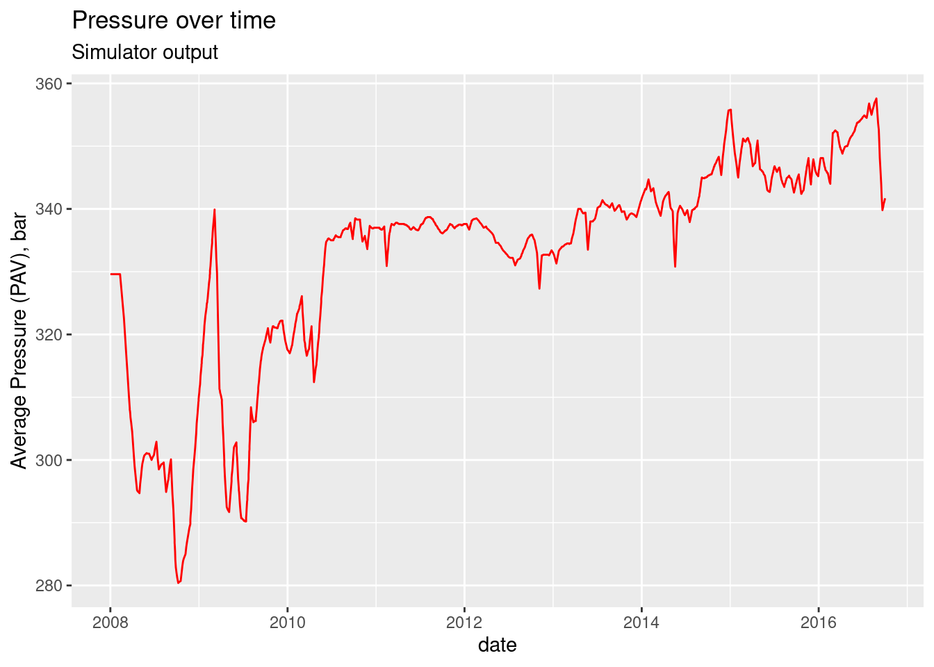
Plot watercut vs time
# plot from PRT simulator output (STEP block)
ggplot(step_info, aes(x =date, y = wct_pct)) +
    geom_line(color = "blue") +
    labs(title = "Field watercut over time", subtitle = "Simulator output",
         y = "Watercut, percent")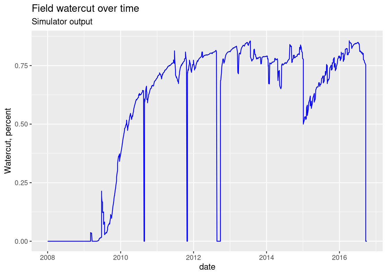
Plot all variables from STEP block
To prevent cluttering our report from lots of plots, we will show all plots in one figure using facets. In order to achieve this, we will have to transform our data in tidy format.
library(tidyr)

# convert to tidy format
step_info_gather <-
step_info %>%
  select(-c(step, time_days)) %>%
  gather(key = var, value, pav_bar:wgr_m3m3) %>%
  print()
#> # A tibble: 6,440 × 3
#>    date       var     value
#>    <date>     <chr>   <dbl>
#>  1 2008-01-01 pav_bar  330.
#>  2 2008-01-01 pav_bar  330.
#>  3 2008-01-02 pav_bar  330.
#>  4 2008-01-03 pav_bar  330.
#>  5 2008-01-05 pav_bar  330.
#>  6 2008-01-08 pav_bar  330.
#>  7 2008-01-11 pav_bar  330.
#>  8 2008-01-14 pav_bar  330.
#>  9 2008-01-17 pav_bar  330.
#> 10 2008-01-21 pav_bar  330.
#> # … with 6,430 more rows
# plot production variables from the STEP block in the PRT file

# change the name of the facet labels
facet_labels <- c(`gor_m3m3` = "GOR, m3/m3", `pav_bar` = "Avg.Pres, bar",
                  `wct_pct` = "Watercut, %", `wgr_m3m3` = "Water Gas Ratio, m3/m3")

# plot the facets with free y-axis.
ggplot(step_info_gather, aes(x = date, y = value)) +
  geom_line() +
  facet_wrap(.~var, scales = "free_y", labeller = as_labeller(facet_labels)) +
  labs(title = "Production variables from STEP block",
       subtitle = "Simulator output", y = "", x = "")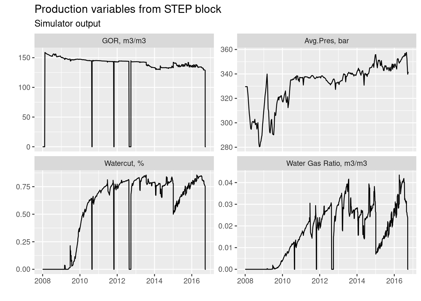
Merge cumulative oil with simulator steps
Next step is combining the data from the steps dataframe with the balance-at production cumulatives. This is not an straight operation since both dataframes have different date references.
First, we will extract the production cumulatives (field totals) from the PRT file. This is something we already did in the previous article. We will load that script.
Save the production cumulatives dataframe as a CSV file.
Join the field_totals and step_info dataframe by a common variable.
Plot variables
Calculate cumulatives
Fix the dates in the merge dataframe so they are continuous from 2018 till October 2016.
Calculate cumulatives and volumes by month
Extract Field cumulatives from the BALANCE-AT block
# load a script with functions
r_folder <- file.path(proj_root, "R")
r_script <- file.path(r_folder, "extract_data_from_prt.R")
source(r_script)

# run function to extract field totals or cumulative production
field_totals <- extract_field_totals(prt_file_content = volve_2016_txt)
field_totals
#> # A tibble: 340 × 8
#>    date        days     ocip     ooip oil_otw wat_otw  gas_otw   pav
#>    <date>     <int>    <dbl>    <dbl>   <dbl>   <dbl>    <dbl> <dbl>
#>  1 2007-12-31     0 21967455 21967455       0       0        0  330.
#>  2 2008-01-11    11 21967456 21967455       0       0        0  330.
#>  3 2008-01-21    21 21967455 21967455       0       0        0  330.
#>  4 2008-01-31    31 21967454 21967455       0       0        0  330.
#>  5 2008-02-10    41 21967454 21967455       0       0        0  330.
#>  6 2008-02-20    51 21948189 21967455   19265       0  3055593  325.
#>  7 2008-02-26    57 21936614 21967455   30840       0  4884638  323.
#>  8 2008-03-01    61 21925419 21967455   42035       0  6650055  320.
#>  9 2008-03-11    71 21897024 21967455   70430       0 11113293  314.
#> 10 2008-03-21    81 21867231 21967455  100223       1 15777548  308.
#> # … with 330 more rows
Save field totals to data files
# save the data
data_folder <- file.path(proj_root, "data")
save(field_totals, file = file.path(data_folder, "field_totals_balance.Rdata"))
write.csv(field_totals, file = file.path(data_folder,
                                         "field_totals_balance.CSV"),
          row.names = FALSE)
We quickly plot the water outflow over the years.
Note. This data might not correct. The PRT file does not explicitely assign a variable for the water outflow. Besides, this volume comes with a negative sign, which indicates injection rather than water production.
# plot from PRT simulator output (BALANCE AT block)
ggplot(field_totals, aes(x =date, y = wat_otw)) +
    geom_line(color = "blue") +
    labs(title = "Field Water Outflow Through Wells",
         subtitle = "Simulator output, BALANCE block",
         y = "Water volume, sm3")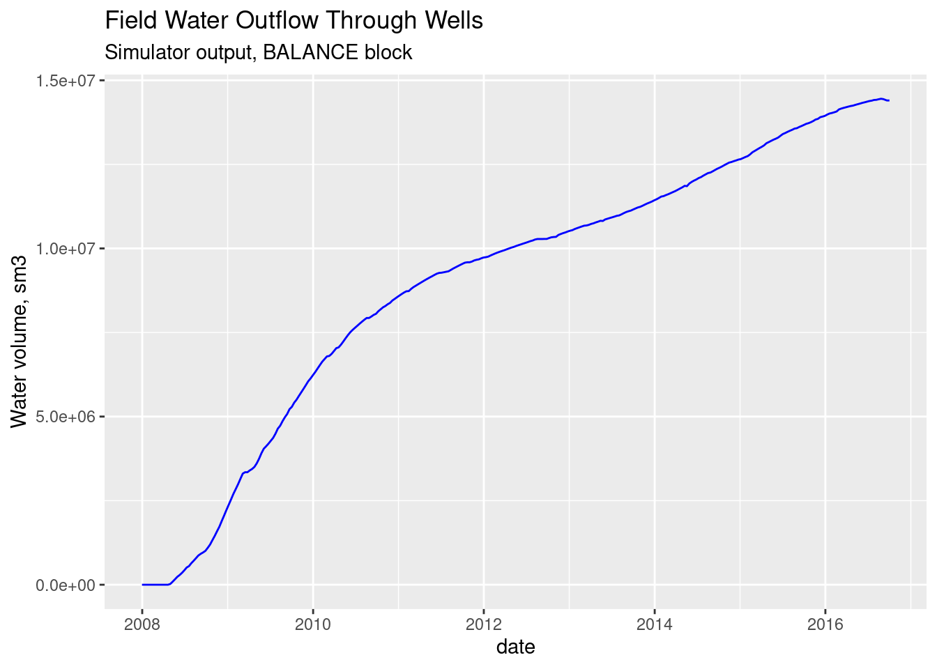
Now, we know that the STEP dataframe has more rows than the BALANCE-AT dataframe. What we want is to correlate the step with the oil cumulatives.
These are the rows in the step_info dataframe:
dim(step_info)
#> [1] 1610    7
These are the number of rows and colums of the field_totals dataframe.
dim(field_totals)
#> [1] 340   8
Join field totals and step dataframes
We merge both tables, steps and field cumulatives. The resultant dataframe we call it step_totals.
# join both tables by the common variable "date"
step_totals <-
left_join(step_info, field_totals, by = "date") %>%
    na.omit() %>%
    select(date, time_days, days, everything()) %>%
    as_tibble() %>%
    print
#> # A tibble: 524 × 14
#>    date       time_days  days  step pav_bar wct_pct gor_m3m3 wgr_m3m3     ocip
#>    <date>         <dbl> <int> <int>   <dbl>   <dbl>    <dbl>    <dbl>    <dbl>
#>  1 2008-01-11      11      11     7    330.       0       0         0 21967456
#>  2 2008-01-21      21      21    10    330.       0       0         0 21967455
#>  3 2008-01-31      31      31    13    330.       0       0         0 21967454
#>  4 2008-02-10      41      41    15    330.       0       0         0 21967454
#>  5 2008-02-20      51      51    17    325.       0     158.        0 21948189
#>  6 2008-02-26      57      57    18    323.       0     158.        0 21936614
#>  7 2008-03-01      61      61    19    320.       0     158.        0 21925419
#>  8 2008-03-11      71      71    21    314.       0     157.        0 21897024
#>  9 2008-03-21      81      81    23    308.       0     156.        0 21867231
#> 10 2008-03-21      81.5    81    24    308        0     156.        0 21867231
#> # … with 514 more rows, and 5 more variables: ooip <dbl>, oil_otw <dbl>,
#> #   wat_otw <dbl>, gas_otw <dbl>, pav <dbl>
The dataframe step_totals has 524 rows or observations and 14 columns or variables.
Looking at this dataframe closer we observe that the date intervals is not uniform; it is not weekle, bi-weekly or monthly because it is a merged dataframe. What we will do next is transforming this dataframe to a monthly summary or where the date intervals is a month separation.
Plot outflow through wells from simulator
Without additional data transformations we plot the cumulatives of the merged dataset.
ggplot(step_totals, aes(x = date, y = oil_otw)) +
    geom_line(color = "dark green", size = 1.1) +
    ggtitle("Cumulative Oil, sm3", subtitle = "Simulator")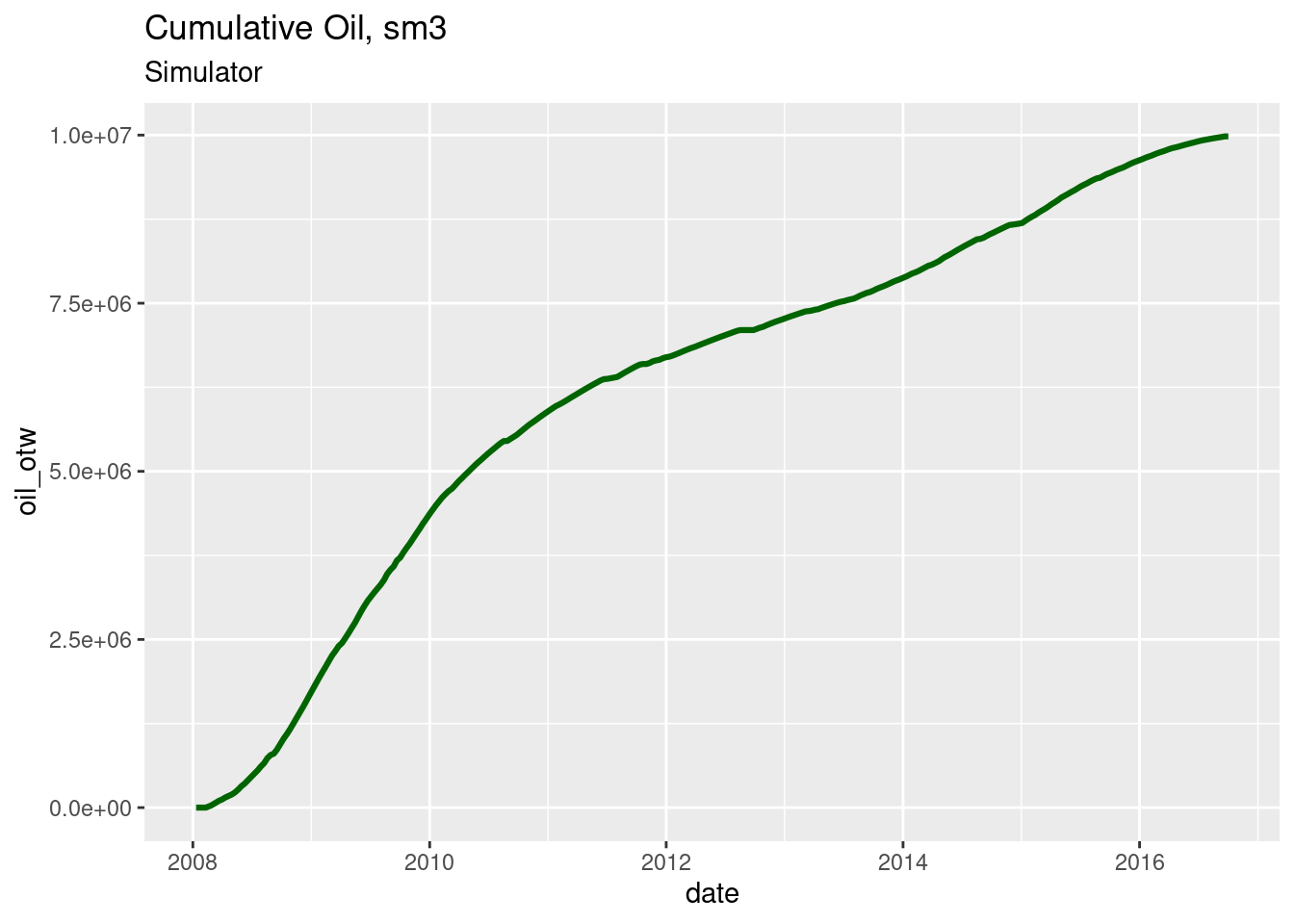
This ggplot for the cumulative gas.
ggplot(step_totals, aes(x = date, y = gas_otw)) +
    geom_line(color = "orange", size = 1.1) +
    labs(title = "Cumulative Gas", subtitle = "Simulator",
         y = "Cumulative Gas, sm3")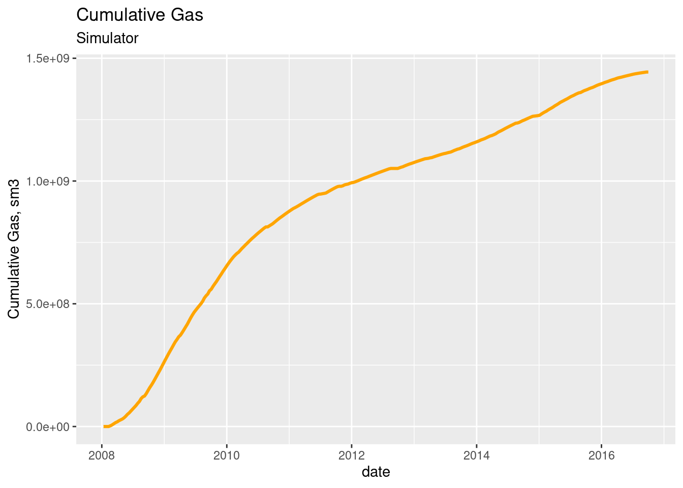
And this another one for cumulative water.
Let’s just keep in mind that this curve may not be right because we are extracting from an incorrect labeled column (water outflow from wells).
ggplot(step_totals, aes(x = date, y = wat_otw)) +
    geom_line(color = "blue", size = 1.1) +
    labs(title = "Cumulative Water", subtitle = "Simulator",
         y = "Cumulative Water, sm3")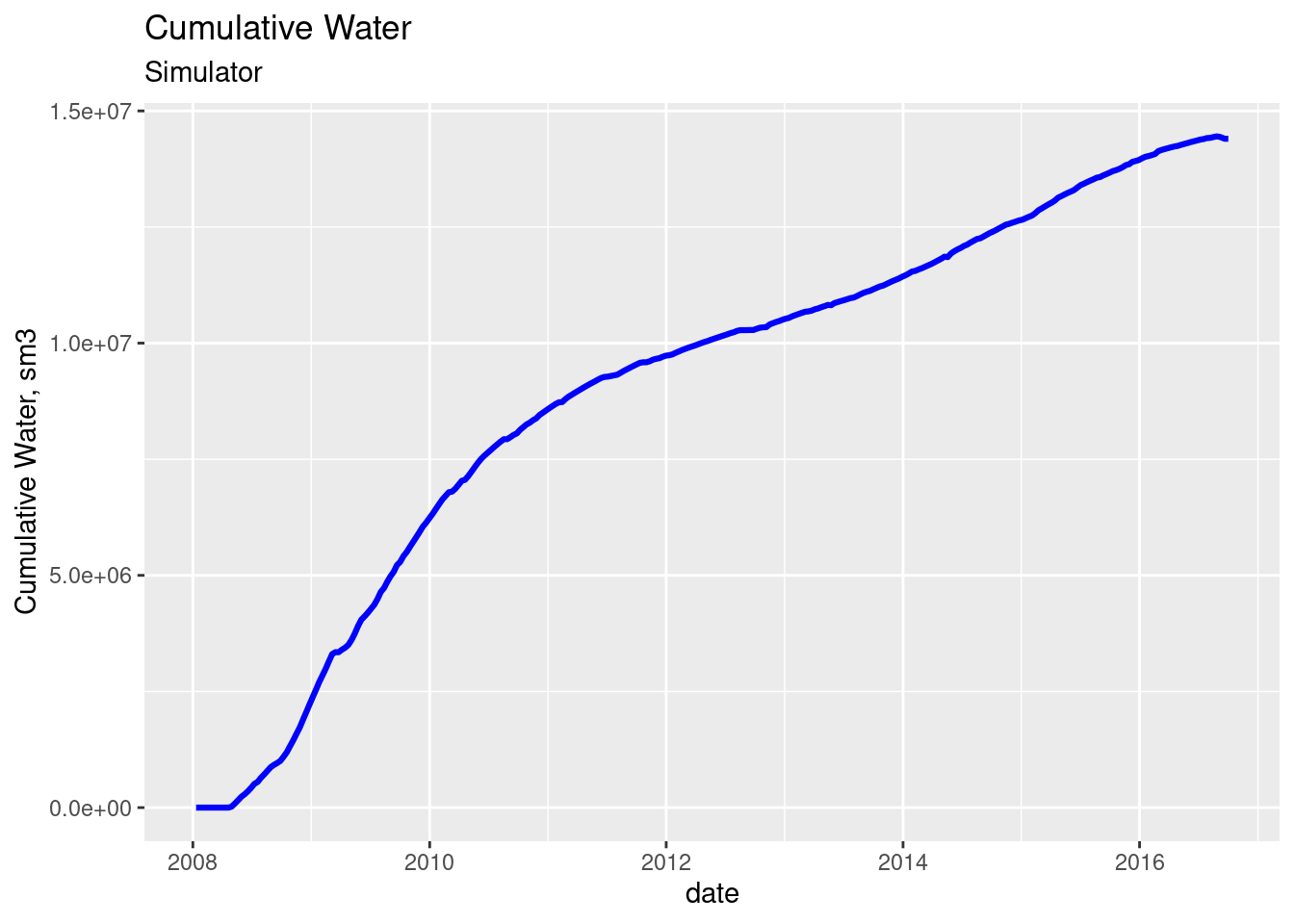
Calculate cumulatives for oil, gas and water for monthly period
This is where we transform the dataframe from an heterogeneous date steps to monthly periods. We use the group_by function operating on the year and the month. This operation, in the end, brings us to a more organized table with a periodic variation. The extra work is recalculating the volumes and cumulatives on the new monthly basis. All these series of transformations are very common when you merge dataframes with different number of rows. What is happening here is:
- calculating the volume at the current period, which is the difference between the current row and the previous one. Wee do that with the lag function.
- decomposing the date in year and month
- grouping by year and month
- summarize the data calculating the volumes per month
- convert the (year, month) to (year, month, day) date format
# step field totals
sim_cumulatives <-
step_totals %>%
    select(date, oil_otw, gas_otw, wat_otw) %>%
    mutate(oil_this_period = oil_otw - lag(oil_otw, default = 0)) %>%
    mutate(gas_this_period = gas_otw - lag(gas_otw, default = 0)) %>%
    mutate(wat_this_period = wat_otw - lag(wat_otw, default = 0)) %>%
    mutate(year = year(date), month = month(date)) %>%
    group_by(year, month) %>%
    summarize(vol_oil = sum(oil_this_period),
              vol_gas = sum(gas_this_period),
              vol_wat = sum(wat_this_period)) %>%
    ungroup() %>%
    mutate(date = ymd(paste(year, month, "01", sep = "-"))) %>%
    # mutate(source = "simulator") %>%
    mutate(cum_oil = cumsum(vol_oil),
           cum_gas = cumsum(vol_gas),
           cum_wat = cumsum(vol_wat)) %>%
    select(date, year, month, everything()) %>%
    print()
#> # A tibble: 106 × 9
#>    date        year month vol_oil  vol_gas vol_wat cum_oil   cum_gas cum_wat
#>    <date>     <dbl> <dbl>   <dbl>    <dbl>   <dbl>   <dbl>     <dbl>   <dbl>
#>  1 2008-01-01  2008     1       0        0       0       0         0       0
#>  2 2008-02-01  2008     2   30840  4884638       0   30840   4884638       0
#>  3 2008-03-01  2008     3   90029 14117066       1  120869  19001704       1
#>  4 2008-04-01  2008     4   73833 11469357   22292  194702  30471061   22293
#>  5 2008-05-01  2008     5  124196 19115952  212550  318898  49587013  234843
#>  6 2008-06-01  2008     6  137247 20967327  192961  456145  70554340  427804
#>  7 2008-07-01  2008     7  155664 24005385  212739  611809  94559725  640543
#>  8 2008-08-01  2008     8  170057 26420155  227653  781866 120979880  868196
#>  9 2008-09-01  2008     9  163015 25205884  137169  944881 146185764 1005365
#> 10 2008-10-01  2008    10  221230 33570835  317736 1166111 179756599 1323101
#> # … with 96 more rows
Filling the date gaps with periodic dates
In this case, at first sight, it seems that we got periodic dates for the production of the field. But what if we are missing a month or two? One way to ensure we have all months accounted for is building a known sequence of dates from 2016-01-01 until 2008-10-01. That is what we do with the function seq.Date():
seq.Date(as.Date("2008-01-01"), as.Date("2016-10-01"), by = "month")
# create a dataframe with complete dates from 2008 until Oct-2016
# this will fill any holes in the dates of any of the two dataframes
dates_complete <- as_tibble(data.frame(date= seq.Date(as.Date("2008-01-01"),
                                          as.Date("2016-10-01"), by = "month"),
                 cum_oil = 0, cum_gas = 0, cum_wat = 0))
dates_complete
#> # A tibble: 106 × 4
#>    date       cum_oil cum_gas cum_wat
#>    <date>       <dbl>   <dbl>   <dbl>
#>  1 2008-01-01       0       0       0
#>  2 2008-02-01       0       0       0
#>  3 2008-03-01       0       0       0
#>  4 2008-04-01       0       0       0
#>  5 2008-05-01       0       0       0
#>  6 2008-06-01       0       0       0
#>  7 2008-07-01       0       0       0
#>  8 2008-08-01       0       0       0
#>  9 2008-09-01       0       0       0
#> 10 2008-10-01       0       0       0
#> # … with 96 more rows
So, there are 106 months from start to end of production.
Next, we proceed to merge the dataframe of known dates (above) with the dataframe sim_cumulatives that we obtained above. Finally, we calculate the volumes and cumulatives.
# simulator production
# merge incomplete dataframe and fill with complete dates
# there will be blank rows or NAs where previously was not data
sim_cumulatives_dt <-
left_join(dates_complete, sim_cumulatives, by = "date") %>%
    # remove NAs from the cumulatives .y
    tidyr::replace_na(list(cum_oil.y = 0, vol_oil = 0,
                           cum_gas.y = 0, vol_gas = 0,
                           cum_wat.y = 0, vol_wat = 0)) %>%        # replace NAs with zeros
    # add up cumulatives .x and .y
    mutate(cum_oil = cum_oil.x + cum_oil.y,
           cum_gas = cum_gas.x + cum_gas.y,
           cum_wat = cum_wat.x + cum_wat.y) %>%       # sum cumulatives
    select(date, cum_oil, cum_gas, cum_wat, vol_oil, vol_gas, vol_wat) %>%
    # replace 0s with previous cumulative. these were rows that didn't exist
    mutate(cum_oil = ifelse(cum_oil == 0, lag(cum_oil, default = 0), cum_oil)) %>%
    mutate(cum_gas = ifelse(cum_gas == 0, lag(cum_gas, default = 0), cum_gas)) %>%
    mutate(cum_wat = ifelse(cum_wat == 0, lag(cum_wat, default = 0), cum_wat)) %>%
    mutate(vol_oil = ifelse(vol_oil == 0, lag(vol_oil, default = 0), vol_oil)) %>%
    mutate(vol_gas = ifelse(vol_gas == 0, lag(vol_gas, default = 0), vol_gas)) %>%
    mutate(vol_oil = ifelse(vol_wat == 0, lag(vol_wat, default = 0), vol_wat)) %>%
    as_tibble() %>%
    print
#> # A tibble: 106 × 7
#>    date       cum_oil   cum_gas cum_wat vol_oil  vol_gas vol_wat
#>    <date>       <dbl>     <dbl>   <dbl>   <dbl>    <dbl>   <dbl>
#>  1 2008-01-01       0         0       0       0        0       0
#>  2 2008-02-01   30840   4884638       0       0  4884638       0
#>  3 2008-03-01  120869  19001704       1       1 14117066       1
#>  4 2008-04-01  194702  30471061   22293   22292 11469357   22292
#>  5 2008-05-01  318898  49587013  234843  212550 19115952  212550
#>  6 2008-06-01  456145  70554340  427804  192961 20967327  192961
#>  7 2008-07-01  611809  94559725  640543  212739 24005385  212739
#>  8 2008-08-01  781866 120979880  868196  227653 26420155  227653
#>  9 2008-09-01  944881 146185764 1005365  137169 25205884  137169
#> 10 2008-10-01 1166111 179756599 1323101  317736 33570835  317736
#> # … with 96 more rows
The negative volume of water and oil are possibly volume corrections by the operator.
# show observations with negative volumes
sim_cumulatives_dt %>%
  filter(vol_oil <0 | vol_wat < 0 | vol_gas < 0)
#> # A tibble: 2 × 7
#>   date       cum_oil    cum_gas  cum_wat vol_oil vol_gas vol_wat
#>   <date>       <dbl>      <dbl>    <dbl>   <dbl>   <dbl>   <dbl>
#> 1 2016-09-01 9980819 1443979050 14400379  -50860 2640331  -50860
#> 2 2016-10-01 9980819 1443979050 14400379  -50860 2640331       0
Comparative of simulator vs historical production
The last step is reading the historical production and compare them against the numbers from the simulation. We start by reading the historical production.
Reading the historical production
Like we did in the previous article, we read the production history from an Excel file. But this time we will be reading all the variables in the dataset.
# load historical production from Excel file
library(xlsx)   # library to read Excel files in R

# read the Excel file
xl_file <- file.path(proj_root, "inst/rawdata", "Volve production data.xlsx")
# read only the monthly production
prod_hist <- as_tibble(read.xlsx(xl_file, sheetName = "Monthly Production Data"))
prod_hist
#> # A tibble: 529 × 10
#>    Wellbore.name NPDCode  Year Month On.Stream Oil   Gas   Water GI    WI
#>    <chr>           <dbl> <dbl> <dbl> <chr>     <chr> <chr> <chr> <chr> <chr>
#>  1 15/9-F-4         5693  2007     9 NULL      NULL  NULL  NULL  NULL  NULL
#>  2 15/9-F-5         5769  2007     9 NULL      NULL  NULL  NULL  NULL  NULL
#>  3 15/9-F-4         5693  2007    10 NULL      NULL  NULL  NULL  NULL  NULL
#>  4 15/9-F-5         5769  2007    10 NULL      NULL  NULL  NULL  NULL  NULL
#>  5 15/9-F-4         5693  2007    11 NULL      NULL  NULL  NULL  NULL  NULL
#>  6 15/9-F-5         5769  2007    11 NULL      NULL  NULL  NULL  NULL  NULL
#>  7 15/9-F-4         5693  2007    12 NULL      NULL  NULL  NULL  NULL  NULL
#>  8 15/9-F-5         5769  2007    12 NULL      NULL  NULL  NULL  NULL  NULL
#>  9 15/9-F-4         5693  2008     1 0         NULL  NULL  NULL  NULL  NULL
#> 10 15/9-F-5         5769  2008     1 0         NULL  NULL  NULL  NULL  NULL
#> # … with 519 more rows
Save raw production history to data files
Once we read the data from Excel we save it as a more standard format: CSV. But this saved data will be very raw because we haven’t performed any operation yet. That’s why we named it production_history_raw.CSV.
# save historical data as raw
data_folder <- file.path(proj_root, "data")
save(prod_hist, file = file.path(data_folder, "production_history_raw.Rdata"))
write.csv(prod_hist, file = file.path(data_folder,
                                         "production_history_raw.CSV"),
          row.names = FALSE)
Cumulatives from production history
These are the data transformations we will perform over the raw production data.
- convert from character to double, integer
- replace the NAs with zeros
- discard two columns with no meaningful data
- rename the variables to all lowercase (easier to remember)
- remove rows that have NAs
- group by year and month
- summarize by volumes
- convert date from character to date format
- sort the data by date
- keep the variables we require
- calculate the cumulatives from volumes
hist_cumulatives <-
prod_hist %>%
    mutate(Oil = as.double(as.character(Oil))) %>%
    mutate(Gas = as.double(as.character(Gas))) %>%
    mutate(Water = as.double(as.character(Water))) %>%
    mutate(Year = as.integer(as.character(Year))) %>%
    mutate(Month = as.integer(as.character(Month))) %>%
    mutate(GI = as.double(as.character(GI))) %>%
    mutate(WI = as.double(as.character(WI))) %>%
    tidyr::replace_na(list(GI = 0, WI = 0)) %>%
    select(-c(NPDCode, On.Stream)) %>%
    rename(year = Year, month = Month, oil = Oil, gas = Gas, wat = Water) %>%
    na.omit() %>%                 # remove all rows that have at least one NA
    group_by(year, month) %>%
    summarise(vol_oil = sum(oil), vol_gas = sum(gas), vol_wat = sum(wat),
              vol_gi = sum(GI), vol_wi = sum(WI)) %>%
    mutate(date = ymd(paste(year, month, "01", sep = "-"))) %>%
    arrange(date) %>%
    ungroup() %>%
    select(date, vol_oil, vol_gas, vol_wat, vol_gi, vol_wi) %>%
    mutate(cum_oil = cumsum(vol_oil), cum_gas = cumsum(vol_gas),
           cum_wat = cumsum(vol_wat),
           cum_gi = cumsum(vol_gi), cum_wi = cumsum(vol_wi)) %>%
    print()
#> # A tibble: 104 × 11
#>    date       vol_oil   vol_gas vol_wat vol_gi vol_wi  cum_oil   cum_gas cum_wat
#>    <date>       <dbl>     <dbl>   <dbl>  <dbl>  <dbl>    <dbl>     <dbl>   <dbl>
#>  1 2008-02-01  49091.  7068009.   413.       0      0   49091.    7.07e6    413.
#>  2 2008-03-01  83361. 12191171.    27.4      0      0  132452.    1.93e7    440.
#>  3 2008-04-01  74532. 11506441.   482.       0      0  206985.    3.08e7    922.
#>  4 2008-05-01 125479. 19091872. 16280.       0      0  332463.    4.99e7  17202.
#>  5 2008-06-01 143787. 21512334.   474.       0      0  476250.    7.14e7  17677.
#>  6 2008-07-01 166280. 24655303.   416.       0      0  642530.    9.60e7  18093.
#>  7 2008-08-01 165444. 23923541.   577.       0      0  807974.    1.20e8  18669.
#>  8 2008-09-01 192263. 27526459.   464.       0      0 1000237.    1.47e8  19134.
#>  9 2008-10-01 237174. 33757700.   725.       0      0 1237411.    1.81e8  19859.
#> 10 2008-11-01 250325. 35743142.  2580.       0      0 1487736.    2.17e8  22439.
#> # … with 94 more rows, and 2 more variables: cum_gi <dbl>, cum_wi <dbl>
Observe that we’ve got 104 rows, which wouldn’t match the rows from the simulation data. We have to fix that. The problem is primarily dates.
Save historical cumulatives as-is
This saves the production history dataframe after the data transformations.
# save historical data
data_folder <- file.path(proj_root, "data")
save(hist_cumulatives, file = file.path(data_folder, "hist_cumulatives_104.Rdata"))
write.csv(hist_cumulatives, file = file.path(data_folder,
                                         "hist_cumulatives_104.CSV"),
          row.names = FALSE)
# create a dataframe with complete dates from 2008 until Oct-2016
df <- as_tibble(data.frame(date= seq.Date(as.Date("2008-01-01"),
as.Date("2016-10-01"), by = "month"),
cum_oil = 0, cum_gas = 0, cum_wat = 0))
df
#> # A tibble: 106 × 4
#> date cum_oil cum_gas cum_wat
#> <date> <dbl> <dbl> <dbl>
#> 1 2008-01-01 0 0 0
#> 2 2008-02-01 0 0 0
#> 3 2008-03-01 0 0 0
#> 4 2008-04-01 0 0 0
#> 5 2008-05-01 0 0 0
#> 6 2008-06-01 0 0 0
#> 7 2008-07-01 0 0 0
#> 8 2008-08-01 0 0 0
#> 9 2008-09-01 0 0 0
#> 10 2008-10-01 0 0 0
#> # … with 96 more rowsRemember that we created this date sequence above. This sequence had 106 rows.
dates_complete
#> # A tibble: 106 × 4
#>    date       cum_oil cum_gas cum_wat
#>    <date>       <dbl>   <dbl>   <dbl>
#>  1 2008-01-01       0       0       0
#>  2 2008-02-01       0       0       0
#>  3 2008-03-01       0       0       0
#>  4 2008-04-01       0       0       0
#>  5 2008-05-01       0       0       0
#>  6 2008-06-01       0       0       0
#>  7 2008-07-01       0       0       0
#>  8 2008-08-01       0       0       0
#>  9 2008-09-01       0       0       0
#> 10 2008-10-01       0       0       0
#> # … with 96 more rows
Fill the dates gap in the production history dataframe
We do almost the same data transformations as before:
- replace NAs in the variables with zeros
- sum up the additional cumulative variables generated during the merge
- replace a cumulative of zero by the previous cumulative (carry over). There cannot be cumulatives of zeros in between. That anomaly is caused by the absence of rows.
- clean up the variables for gas injection (GI) and water injection (WI) volumes
- calculate the cumulatives for gas injection and water injection
# historical production
# merge incomplete dataframe and complete with dates
hist_cumulatives_dt <-
left_join(dates_complete, hist_cumulatives, by = "date") %>%
    # replace NAs with zeros
    tidyr::replace_na(list(cum_oil.y = 0, cum_gas.y = 0, cum_wat.y = 0)) %>%
    tidyr::replace_na(list(vol_oil = 0, vol_gas = 0, vol_wat = 0)) %>%
    tidyr::replace_na(list(vol_gi = 0, vol_wi = 0, cum_gi = 0, cum_wi = 0)) %>%
    # add up the extra column .y
    mutate(cum_oil = cum_oil.x + cum_oil.y) %>%
    mutate(cum_gas = cum_gas.x + cum_gas.y) %>%
    mutate(cum_wat = cum_wat.x + cum_wat.y) %>%
    # filter(date != as.Date("2016-10-01")) %>%
    # this fixes the zeros generated by adding complete dates
    mutate(cum_oil = ifelse(cum_oil == 0, lag(cum_oil, default=0), cum_oil)) %>%
    mutate(cum_gas = ifelse(cum_gas == 0, lag(cum_gas, default=0), cum_gas)) %>%
    mutate(cum_wat = ifelse(cum_wat == 0, lag(cum_wat, default=0), cum_wat)) %>%
    mutate(cum_gi = ifelse(cum_gi == 0, lag(cum_gi, default=0), cum_gi)) %>%
    mutate(cum_wi = ifelse(cum_wi == 0, lag(cum_wi, default=0), cum_wi)) %>%
    select(date, cum_oil, cum_gas, cum_wat, vol_oil, vol_gas, vol_wat,
           vol_gi, vol_wi, cum_gi, cum_wi) %>%
    as_tibble() %>%
    print
#> # A tibble: 106 × 11
#>    date        cum_oil    cum_gas cum_wat vol_oil  vol_gas vol_wat vol_gi vol_wi
#>    <date>        <dbl>      <dbl>   <dbl>   <dbl>    <dbl>   <dbl>  <dbl>  <dbl>
#>  1 2008-01-01       0          0       0       0    0          0        0      0
#>  2 2008-02-01   49091.   7068009.    413.  49091.   7.07e6   413.       0      0
#>  3 2008-03-01  132452.  19259180.    440.  83361.   1.22e7    27.4      0      0
#>  4 2008-04-01  206985.  30765621.    922.  74532.   1.15e7   482.       0      0
#>  5 2008-05-01  332463.  49857492.  17202. 125479.   1.91e7 16280.       0      0
#>  6 2008-06-01  476250.  71369826.  17677. 143787.   2.15e7   474.       0      0
#>  7 2008-07-01  642530.  96025129.  18093. 166280.   2.47e7   416.       0      0
#>  8 2008-08-01  807974. 119948670.  18669. 165444.   2.39e7   577.       0      0
#>  9 2008-09-01 1000237. 147475129.  19134. 192263.   2.75e7   464.       0      0
#> 10 2008-10-01 1237411. 181232829.  19859. 237174.   3.38e7   725.       0      0
#> # … with 96 more rows, and 2 more variables: cum_gi <dbl>, cum_wi <dbl>
Great! We got the dataframe hist_cumulatives_dt, with 106 rows and 11 columns.
Plot production rates
If we want to plot several variables in one figure we have to convert the dataframe into tidy data format, and then use facets.
hist_cumulatives_dt_gather <-
hist_cumulatives_dt %>%
  select(date, vol_oil, vol_gas, vol_wat) %>%
  gather(key = var, value, vol_oil:vol_wat) %>%

  print()
#> # A tibble: 318 × 3
#>    date       var       value
#>    <date>     <chr>     <dbl>
#>  1 2008-01-01 vol_oil      0
#>  2 2008-02-01 vol_oil  49091.
#>  3 2008-03-01 vol_oil  83361.
#>  4 2008-04-01 vol_oil  74532.
#>  5 2008-05-01 vol_oil 125479.
#>  6 2008-06-01 vol_oil 143787.
#>  7 2008-07-01 vol_oil 166280.
#>  8 2008-08-01 vol_oil 165444.
#>  9 2008-09-01 vol_oil 192263.
#> 10 2008-10-01 vol_oil 237174.
#> # … with 308 more rows
And this is the plot of the cumulative variables from the production history.
# plot production variables from the STEP block in the PRT file

# order of the plots
hist_cumulatives_dt_gather$var_f <-
  factor(hist_cumulatives_dt_gather$var,
         levels = c("vol_oil", "vol_gas", "vol_wat"))

# change the name of the facet labels
facet_labels <- c(`vol_oil` = "Oil", `vol_gas` = "Gas", `vol_wat` = "Water")

ggplot(hist_cumulatives_dt_gather, aes(x = date, y = value, color = var)) +
  geom_line(size = 1) +
  facet_grid(var_f ~., scales = "free_y",
             labeller = as_labeller(facet_labels)) +
  labs(title = "Monthly fluid Volumes, m3",
       subtitle = "Historical Production", y = "", x = "")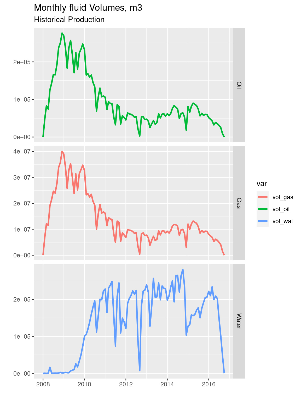
Save historical cumulatives with fixed dates
We save the date fixed production history in CSV format file.
# save historical data with complete dates. 106 rows
data_folder <- file.path(proj_root, "data")
save(hist_cumulatives_dt, file = file.path(data_folder, "hist_cumulatives_dt.Rdata"))
write.csv(hist_cumulatives_dt, file = file.path(data_folder, "hist_cumulatives_dt.CSV"),
          row.names = FALSE)
Plot historical cumulatives of oil, gas and water
library(gridExtra)

# cumulative oil from historical production
p1 <- ggplot(hist_cumulatives_dt, aes(x = date, y = cum_oil)) +
    geom_line() +
    geom_col(color = "dark green", fill = "dark green", alpha = 0.35) +
    ggtitle("Cumulative Oil, sm3", subtitle = "Historical Production")

# cumulative gas from historical production
p2 <- ggplot(hist_cumulatives_dt, aes(x = date, y = cum_gas)) +
    geom_line() +
    geom_col(color = "orange", fill = "orange", alpha = 0.35) +
    ggtitle("Cumulative Gas, sm3", subtitle = "Historical Production")

# cumulative water from historical production
p3 <- ggplot(hist_cumulatives_dt, aes(x = date, y = cum_wat)) +
    geom_line() +
    geom_col(color = "blue", fill = "blue", alpha = 0.35) +
    ggtitle("Cumulative Water, sm3", subtitle = "Historical Production")

grid.arrange(p1, p2, p3, ncol =1)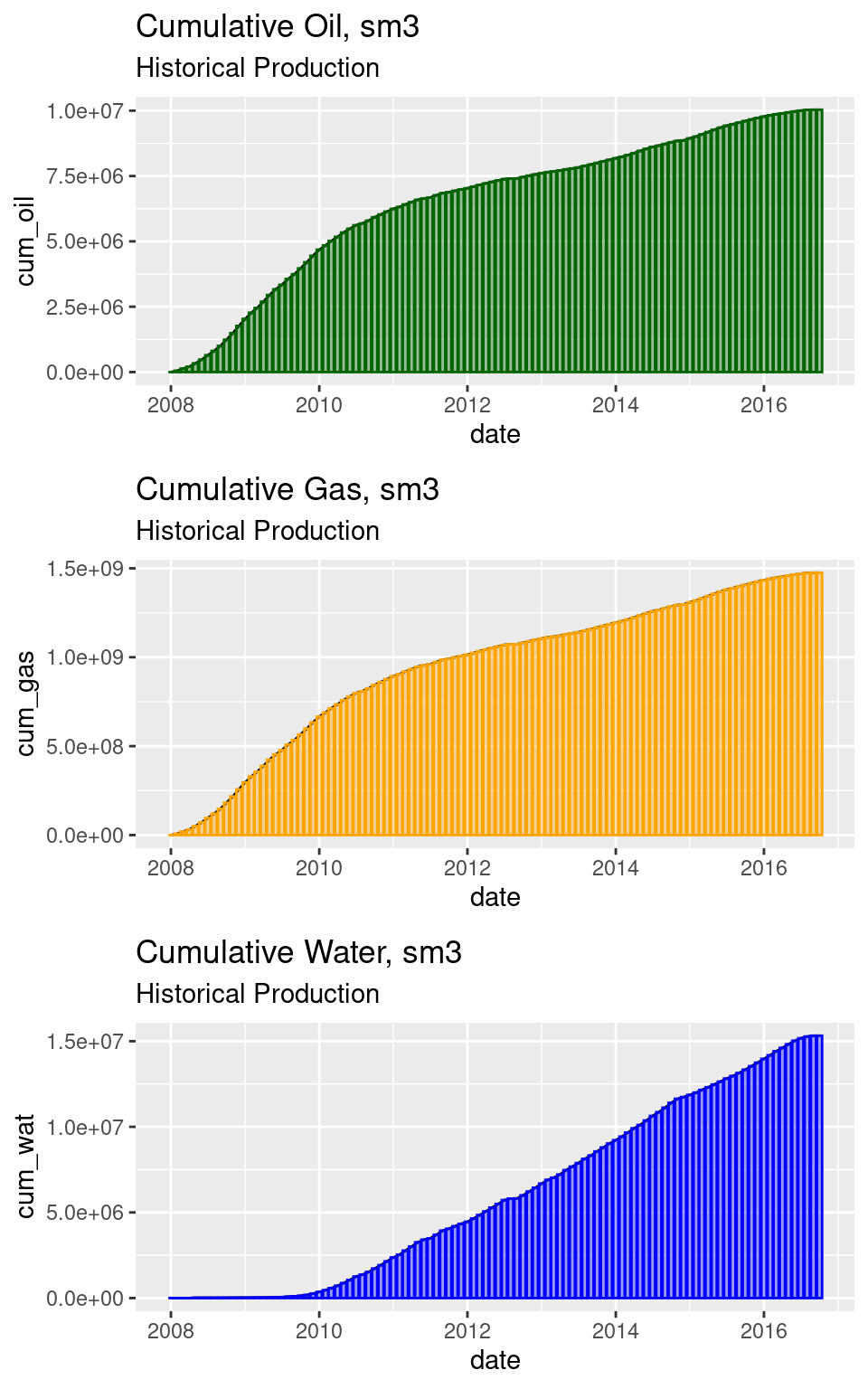
Rename the variables according to source
Finally, because we want to combine the simulation results with the measured production for each fluid, on the same plot, we will rename the variables to something is directly recognizable as the source: simulator or historical.
These are the data transformations:
- rename the variables in the sim_cumulatives_dt dataframe
- rename the variables in the hist_cumulatives_dt dataframe
- join the resulting dataframe by the common variable date
# rename the simulation cumulatives
sim_cumulatives_src <-
sim_cumulatives_dt %>%
    select(date, cum_oil, cum_gas, cum_wat) %>%
    rename(cum_oil_sim = cum_oil, cum_gas_sim = cum_gas, cum_wat_sim = cum_wat)


# rename historical cumulatives according to source
hist_cumulatives_src <-
hist_cumulatives_dt %>%
    select(date, cum_oil, cum_gas, cum_wat) %>%
    rename(cum_oil_hist = cum_oil, cum_gas_hist = cum_gas, cum_wat_hist = cum_wat)

# combine simulator and historical dataframes. common variable is "date"
cumulatives_all <- full_join(hist_cumulatives_src, sim_cumulatives_src, by = "date")
cumulatives_all
#> # A tibble: 106 × 7
#>    date       cum_oil_hist cum_gas_hist cum_wat_hist cum_oil_sim cum_gas_sim
#>    <date>            <dbl>        <dbl>        <dbl>       <dbl>       <dbl>
#>  1 2008-01-01           0            0            0            0           0
#>  2 2008-02-01       49091.     7068009.         413.       30840     4884638
#>  3 2008-03-01      132452.    19259180.         440.      120869    19001704
#>  4 2008-04-01      206985.    30765621.         922.      194702    30471061
#>  5 2008-05-01      332463.    49857492.       17202.      318898    49587013
#>  6 2008-06-01      476250.    71369826.       17677.      456145    70554340
#>  7 2008-07-01      642530.    96025129.       18093.      611809    94559725
#>  8 2008-08-01      807974.   119948670.       18669.      781866   120979880
#>  9 2008-09-01     1000237.   147475129.       19134.      944881   146185764
#> 10 2008-10-01     1237411.   181232829.       19859.     1166111   179756599
#> # … with 96 more rows, and 1 more variable: cum_wat_sim <dbl>
That’s it. Our final comparison dataframe with 106 rows and 7 columns.
Observations
In order to observe how close was the history matching, we plot the cumulative production from the simulator versus that of the historical production. Additionally, we want to shade the are between the two curves to show the difference.
How close cumulative productions are
Cumulative oil. Historical vs simulator
# Volve reservoir model dataset
# plot historical vs simulator cum_oil

# manual assignment of colors in the legend
cols <- c("simulator"="red", "historical"="blue") # legend: colors and names
ggplot(cumulatives_all) +
    # shade the area between the curves
    geom_ribbon(aes(x = date, ymin= cum_oil_sim, ymax= cum_oil_hist),
                fill = "dark green", alpha = 0.35) +
    geom_line(aes(x = date, y = cum_oil_sim, color = "simulator")) +
    geom_line(aes(x = date, y = cum_oil_hist, color = "historical")) +
    labs(title = "Volve reservoir model. Comparison Cumulative Oil",
         subtitle = "Historical vs Simulator",
         y = "cumulative oil, sm3") +
    scale_color_manual(name = "Curve", values = cols)  # manual legend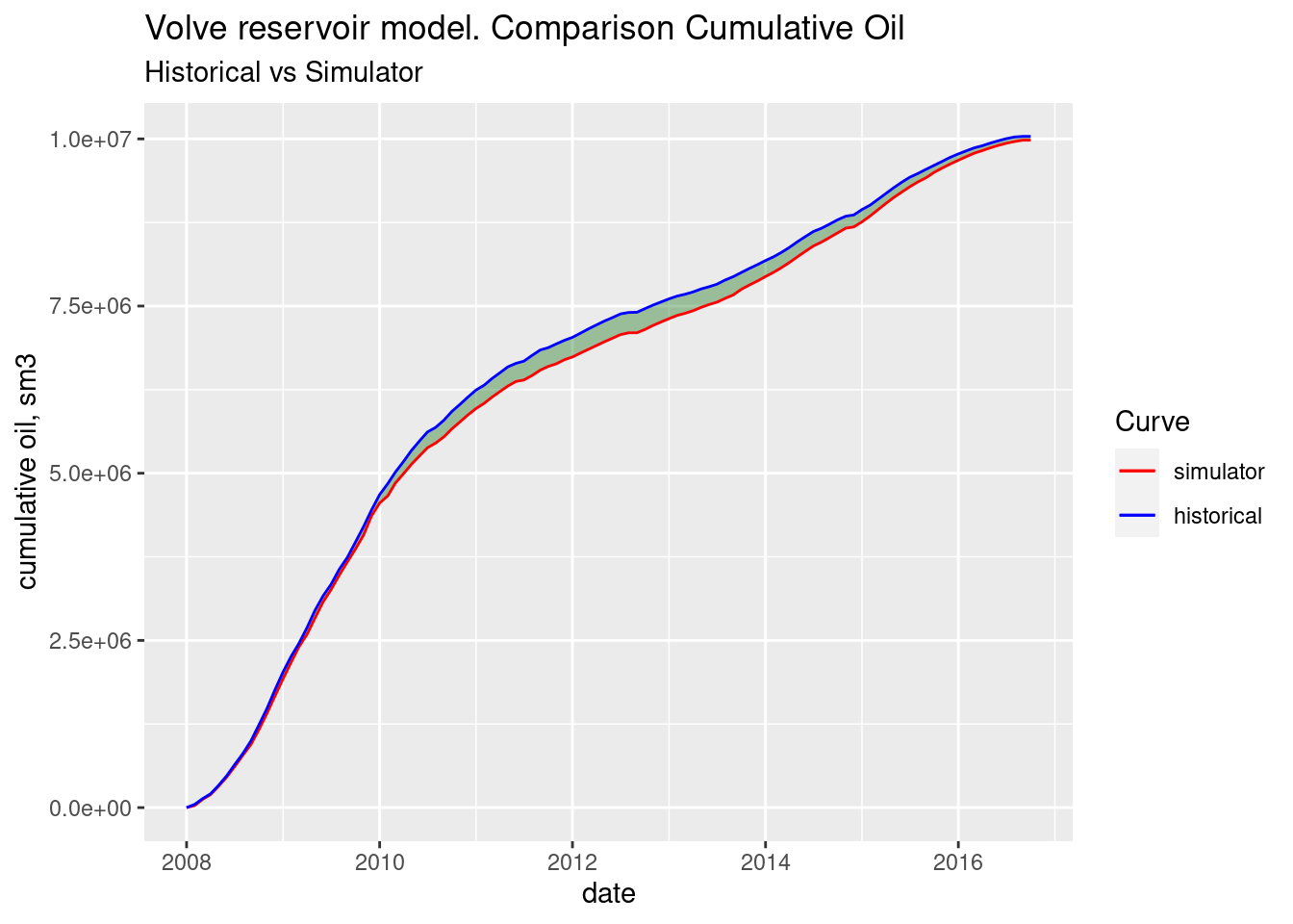
Cumulative gas. Historical vs simulator
# Volve reservoir model dataset
# plot historical vs simulator cum_gas
cols <- c("simulator"="red", "historical"="blue") # legend: colors and names
ggplot(cumulatives_all) +
    # shade the area between the curves
    geom_ribbon(aes(x = date, ymin= cum_gas_sim, ymax= cum_gas_hist),
                fill = "orange", alpha = 0.35) +
    geom_line(aes(x = date, y = cum_gas_sim, color = "simulator"), size = 1) +
    geom_line(aes(x = date, y = cum_gas_hist, color = "historical"), size = 1) +
    labs(title = "Volve reservoir model. Comparison Cumulative Gas",
         subtitle = "Historical vs Simulator",
         y = "cumulative gas, sm3") +
    scale_color_manual(name = "Curve", values = cols)  # manual legend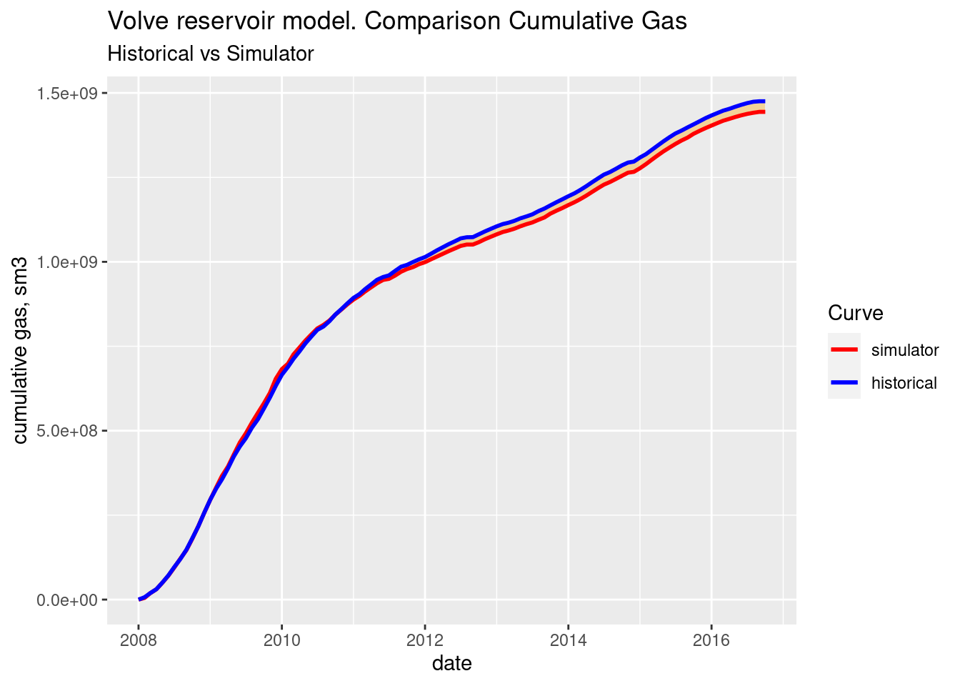
Cumulative water. Historical vs simulator
# Volve reservoir model dataset
# plot historical vs simulator cumulative water variable
cols <- c("simulator"="red", "historical"="blue") # legend: colors and names
ggplot(cumulatives_all) +
    # shade the area between the curves
    geom_ribbon(aes(x = date, ymin= cum_wat_sim, ymax= cum_wat_hist),
                fill = "cyan", alpha = 0.35) +
    geom_line(aes(x = date, y = cum_wat_sim, color = "simulator"), size = 1) +
    geom_line(aes(x = date, y = cum_wat_hist, color = "historical"), size = 1) +
    labs(title = "Volve reservoir model. Comparison Cumulative Water",
         subtitle = "Historical vs Simulator",
         y = "cumulative water, sm3") +
    scale_color_manual(name = "Curve", values = cols)  # manual legend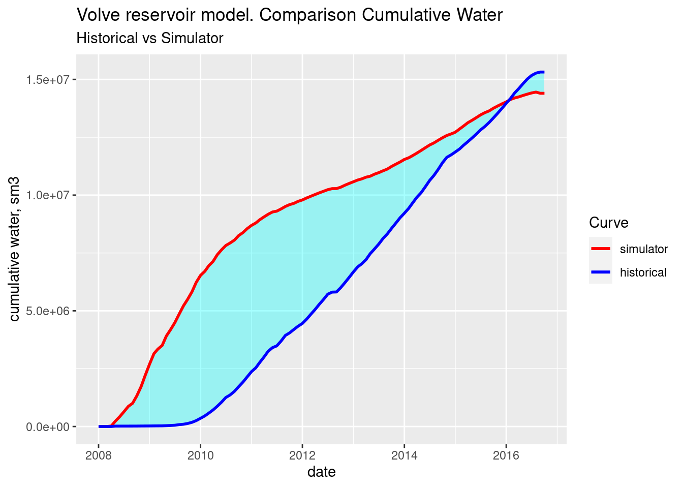
Note. This last plot for the cumulative water has been observed different when another reservoir engineer Konstantin Sermyagin was able to read directly from the Eclipse binary files. I have checked the cumulative water from the simulator and it has been properly extracted and transformed. Still, I have some doubts about the extraction of the cumulative water because the outflow doesn’t seem to originate from connate water but from injection water as well. If you download the Eclipse PRT file, please, take a look at the BALANCE AT blocks. Try to identify the variable corresponding to connate water only. I am not sure why Eclipse does not make a distinction between the two sources of water.
Datasets
Volve 2016 dataset for reservoir simulation model. Compressed PRT output as zip file. Zenodo
data_from_step.CSV: data from STEP block.
field_totals_balance.CSV: save the field totals from BALANCE block.
hist_cumulatives_104.CSV: historical data after data transformations. 104 rows.
hist_cumulatives_dt.CSV: historical data with complete dates. 106 rows.
production_history.CSV: Production history read from Excel file. Raw.