![]()
Introduction
History matching is one of the core activities performed by petroleum engineers to decrease the uncertainty of reservoir models. By comparing real data -production data gathered at the surface-, with the output from a reservoir simulator, the engineer starts filling in the gaps in reservoir properties of those block cells in the model.
And this what makes it so interesting in data science, and ultimately, in the fabrication or construction of an artificial intelligence agent. Why? Because it represents the confluence of a reservoir model -physics based-, and real world data, the production history. Don’t get me wrong here! It is not data science versus physics or engineering. It is about transforming data in a better instrument to improve the quality of the output of the model.
I cannot think of a better example right now to start proving an intelligent agent for reservoir history matching. There is plenty of literature; there are some real and synthetic reservoir models which have been subject of machine learning algorithms extensively in SPE papers. Very good papers indeed. With the only drawback that they cannot be reproduced. The process or algorithm cannot be reproduced outside the original environment in which it was written, or by any other than the original author.
What about if we try a different approach: given that it has been proven that history matching works by introducing machine learning algorithms in the process, let’s pick one or some of them, and try recreating the data science workflow step-by-step: from the raw data (production history and reservoir model output), up to the automatic comparison of the model with the new proposed reservoir data. The workflow should be publicly available so other petroleum engineers could pick up where it is and improving it for their own environment setting. In other words, we will work on making a reproducible example of a reservoir history matching process.
And what better than using a reservoir model already given it to us for free? I am talking about the Volve dataset.
Motivation
For some months now I’ve been reading about applications of machine learning and artificial intelligence for petroleum engineering. There is quite interesting literature in papers - I wrote a quick statistic on the subject of data science, ML and AI that can be found in SPE papers few weeks ago.
Be forewarned though. This will be a common obstacle you will find: although there is a good stream of papers on ML and AI in OnePetro, one of the things those papers are lacking is reproducibility. From approximately 1,000 papers, maybe less than 5 have data, code and report accompanying the paper. At this crossroads of intelligent machines, it looks to me like a major crisis in the petroleum industry.
There cannot be data science without reproducibility; and much less machine learning or artificial intelligence without data science.
In your understanding, how the word “science” comes to be part of “data science”?
Or, what are the inherent characteristics of a science that data science must adopt to be called a science?
Or what makes reproducibility a key part of data science?
Artificial Intelligence agent workflow
Artificial intelligence agents are essentially a product of computer science, math and statistics. There is no magic in it; it just very hard. A bit of a science as well as an art. You can say it is just a new way of coding using data as the raw material for making a machine learn from data. Then, applying an algorithm, or set of algorithms, to make this process cyclical to improve its accuracy with each succesive iteration.
How do we get to this point?
Let’s start first with a simple flow everyday text diagram:
A reservoir model has still some unknowns in its properties
We have a workflow to perform history matching but it is manual, it takes a long time, requires interruption to enter new data or updating it, it could be prone to error when copy-pasting data, it is boring because it needs babysitting during the whole process, and is heartbreaking because if the production history doesn’t match the reservoir simulation output we have to start all over.
We have production history -rates and cumulatives-, that is available every week or at the end of month.
The output of the reservoir model is yet far from matching the real production data
The reservoir simulation may take hours or days to run, or it engaged in another task.
What can we do different to make this matching process learning from data?
I will be making an attempt of building a high level step-by-step recipe based on the reading of relevant papers:
Use a reservoir simulation software to generate a series of outputs at different reservoir properties values within practical range
Extract data from the simulation reports, specifically, production data, rates and cumulatives.
Create a rectangular dataset based on the production output from the simulator and the reservoir properties that were generated as inputs
Correlate the reservoir cells to each of those random generated reservoir properties. Enter x, y, z coordinates for cell and property, as well as well id, area or zone, layer, thickness, etc. Think of it as creating a unique address for each reservoir cell which you will be assigning a new reservoir property.
The reservoir property could be permeability, porosity, saturation, tranmissibility, or any other property that is still unknown. It may be a good idea when you are starting that you practice varying one property at a time. Let’s say permeability, and see how adjusting this property improves the accuracy of your reservoir model. Then, once you get the hang of it, continue adding complexity to the model.
For every set of changes that you make on the reservoir model you will run the simulator to obtain a corresponding output set: a simulation run. It is this report from where you will be extracting the synthetic production data for your dataset.
The dataset is the data source that the machine learning algorithm will use to match synthetic production against real production. The algorithm could be any ML algorithm that you find the best RMSE (Root Mean Squared Error) - the lowest the better.
You may find scenarios in which a combination of reservoir properties yields more than one match. Here we will have to use an optimization method to pick the best combination.
Once we obtain an acceptable set of reservoir properties these are entered in the reservoir model for testing. Extract the output from the reservoir simulator and compare against the production history.
Repeat this process after new production data becomes available.
You will find after some runs of this workflow that it could be automated. You will have to identify the parts in the workflow that are harder to automate or less dependant of supervision. In parallel, several algorithms will have to be identified at critical steps of the process. There is no one algorithm that will do it all.
First steps: the Volve reservoir dataset
Last year Equinor released a huge dataset for the Volve field. Many terabytes of data, approximately 4298 gigabytes of it.
# megabytes
cat(sprintf("Megabytes\n"))
#> Megabytes
(mega <- c(geophysics = 99, reservoir_eclipse = 390, well_technical = 212,
          seismic_vsp = 95, production = 2, reports = 162))
#>        geophysics reservoir_eclipse    well_technical       seismic_vsp
#>                99               390               212                95
#>        production           reports
#>                 2               162
# gigabytes
cat(sprintf("Gigabytes\n"))
#> Gigabytes
(giga <- c(geoscience = 54.6, reservoir_rms = 2.1, well_logs = 6.9,
          seismic_4d = 330.4, well_logs_per_well = 7, witsml_drilling = 5))
#>         geoscience      reservoir_rms          well_logs         seismic_4d
#>               54.6                2.1                6.9              330.4
#> well_logs_per_well    witsml_drilling
#>                7.0                5.0
# terabytes
cat(sprintf("Terabytes\n"))
#> Terabytes
(tera <- c(seismic_st10010 = 2.6, seismic_st0202 = 1.2))
#> seismic_st10010  seismic_st0202
#>             2.6             1.2
# Summary
cat(sprintf("\nDataset in GB\n"))
#>
#> Dataset in GB
c(mega / 1024, giga, tera * 1024)
#>         geophysics  reservoir_eclipse     well_technical        seismic_vsp
#>       9.667969e-02       3.808594e-01       2.070312e-01       9.277344e-02
#>         production            reports         geoscience      reservoir_rms
#>       1.953125e-03       1.582031e-01       5.460000e+01       2.100000e+00
#>          well_logs         seismic_4d well_logs_per_well    witsml_drilling
#>       6.900000e+00       3.304000e+02       7.000000e+00       5.000000e+00
#>    seismic_st10010     seismic_st0202
#>       2.662400e+03       1.228800e+03
giga_total <- sum(c(mega / 1024, giga, tera * 1024))

# how many gigabytes of data?
cat(sprintf("\nTotal Gigabytes: %8.3f", giga_total))
#>
#> Total Gigabytes: 4298.137
For the reservoir simulation part we’ve got 399 megabytes of compressed data, or 1.58 gigabytes of uncompressed files. Most of the files are text files but there are few that are in binary. Text files are easy to access and somewhat difficult to read as structured data. On the other hand, binary files are difficult to read if you don’t know the proper reading format but they come in more structured form.
You may want to sign up for access to the website and download the data files here. Here is a screenshot to the datasets available. Pay special attention to the sizes of the compressed files. The seismic files are gigantic.
#> Error in knitr::include_graphics("/img/volve_datasets.png"): Cannot find the file(s): "/img/volve_datasets.png"I downloaded the datasets using Azure Explorer, a Microsoft utility that makes the download process almost painless. You can download the software here.
The Volve reservoir X-files
From all the files in the reservoir dataset, I will pay particular attention to the VOLVE_2016.PRT file. It is a 233 MB file containing the output of the reservoir simulation.
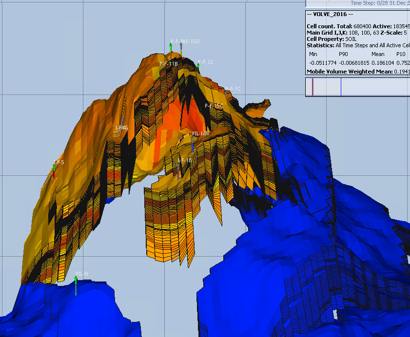
Volve is a field that ended production in 2016 producing for approximately 8.5 years. So, we won’t be doing the history matching with new production history data; we will be using production data from 2008 through 2016. The reservoir model is 108 by 100 by 63 cells. From the 680,400 cells only 183,545 are active. Volves has an Oil Originally in Place (OOIP) of approximately 22 MM m3.
Working with the output of the reservoir simulation is part of a larger process in our path to create an artificial intelligent agent. Let’s start by defining what the goals are:
Read the synthetic production data from the reservoir simulation output
Extract the rates and cumulatives-, and put them in a rectangular dataset, in other words, let’s save the data in a dataframe.
Once the synthetic production data is ready, it is time to read the data from the real production history.
Transform and convert the data to the same units and similar time steps.
Compare the synthetic data vs the real production data.
Observe the differences and evaluate if you have a match.
Read the production data from the reservoir simulator
As we mentioned earlier, we will be reading the data from the output file from the reservoir simulator. This is an output of an Eclipse software.
It will take few seconds to read since it is a 228 megabytes file.
library(dplyr)

# # read the Eclipse report
# proj_root <- rprojroot::find_rstudio_root_file()
# # had to zip the PRT file because 225 MB and too big for Github
# volve_2016_zip <- file.path(proj_root, "inst/rawdata", "VOLVE_2016.zip")
# temp <- tempdir()
#
# volve_2016_txt <- readLines(unzip(volve_2016_zip, exdir = temp))
# download a ZIP file from Google drive
# original share link. Extract the ID of the file
temp <- tempfile(fileext = ".zip")
# provide ID for zip file
gfile_link <- "https://drive.google.com/uc?export=download&id=1rdHuBDWTbykxVkgCgz9e_pp6kUpcrtKT"
download.file(gfile_link, temp, mode = "wb")
volve_2016_txt <- readLines(unzip(temp, exdir = tempdir()))There is one set of data we are interested in: the cumulative production data. This data can be located in the report by using the find tool in the text editor searching for the keyword BALANCE AT.
#> Error in knitr::include_graphics("/img/balance_at-block.png"): Cannot find the file(s): "/img/balance_at-block.png"What we will be reading are the following variables:
- days: elapse days since the start of the simulation.
- date: date in the simulation
- oil currently in place (
ocip) - oil originally in place (
ooip) - gas currently in place (
gcip) - gas originally in place (
goip)
library(dplyr)

# find the rows where we find the word "BALANCE  AT"
balance_rows <- grep("^.*BALANCE  AT", volve_2016_txt)

# add rows ahead to where the word BALANCE AT was found
field_totals_range <- lapply(seq_along(balance_rows), function(x)
    c(balance_rows[x], balance_rows[x]+1:21))

# try different strategy
# iterating through the report pages in FIELD TOTALS
# get:
#    days, oil currently in place, oil originally in place,
#    oil outflow through wells

# get the text from all pages and put them in a list
field_totals_report_txt <- lapply(seq_along(field_totals_range), function(x)
    volve_2016_txt[field_totals_range[[x]]])

# iterate through the list of pages
field_totals_dfs <- lapply(seq_along(field_totals_report_txt), function(x) {
    page <- field_totals_report_txt[[x]]  # put all pages text in a list
    days_row_txt <- page[1] # get 1st row of page
    days_value <- sub(".*?(\\d+.\\d.)+.*", "\\1", days_row_txt) # extract the days
    # get the date
    date_row_txt <- grep("^.*REPORT", page)
    date_value <- sub(".*?(\\d{1,2} [A-Z]{3} \\d{4})+.*", "\\1", page[date_row_txt])
    # get oil currently in place
    ocip_row_txt <- grep("^.*:CURRENTLY IN PLACE", page)
    ocip_value <- sub(".*?(\\d+.)+.*", "\\1", page[ocip_row_txt])
    # get OOIP
    ooip_row_txt <- grep("^.*:ORIGINALLY IN PLACE", page)
    ooip_value <- sub(".*?(\\d+.)+.*", "\\1", page[ooip_row_txt])
    # get total fluid outflow through wells
    otw_row_txt <- grep("^.*:OUTFLOW THROUGH WELLS", page) # row index at this line
    otw_group_pattern <- ".*?(\\d+.)+.*?(\\d+.)+.*?(\\d+.)+.*"  # groups
    oil_otw_value <- sub(otw_group_pattern, "\\1", page[otw_row_txt]) # get oil outflow
    wat_otw_value <- sub(otw_group_pattern, "\\2", page[otw_row_txt]) # get gas outflow
    gas_otw_value <- sub(otw_group_pattern, "\\3", page[otw_row_txt]) # get water
    # get pressure
    pav_row_txt <- grep("PAV =", page)
    pav_value <- sub(".*?(\\d+.\\d.)+.*", "\\1", page[pav_row_txt])
    # dataframe
    data.frame(date = date_value, days = as.double(days_value),
               ocip = as.double(ocip_value),
               ooip = as.double(ooip_value),
               oil_otw = as.double(oil_otw_value),
               wat_otw = as.double(wat_otw_value),
               gas_otw = as.double(gas_otw_value),
               pav = as.double(pav_value),
               stringsAsFactors = FALSE
               )
})

field_totals <- do.call("rbind", field_totals_dfs)
The first 20 rows of the field totals:
head(field_totals, 20)
#>           date days     ocip     ooip oil_otw wat_otw  gas_otw    pav
#> 1  31 DEC 2007    0 21967455 21967455       0       0        0 329.61
#> 2  11 JAN 2008   11 21967456 21967455       0       0        0 329.61
#> 3  21 JAN 2008   21 21967455 21967455       0       0        0 329.62
#> 4  31 JAN 2008   31 21967454 21967455       0       0        0 329.63
#> 5  10 FEB 2008   41 21967454 21967455       0       0        0 329.64
#> 6  20 FEB 2008   51 21948189 21967455   19265       0  3055593 325.21
#> 7  26 FEB 2008   57 21936614 21967455   30840       0  4884638 322.63
#> 8   1 MAR 2008   61 21925419 21967455   42035       0  6650055 320.17
#> 9  11 MAR 2008   71 21897024 21967455   70430       0 11113293 314.17
#> 10 21 MAR 2008   81 21867231 21967455  100223       1 15777548 308.19
#> 11 31 MAR 2008   91 21846585 21967455  120869       1 19001704 304.49
#> 12 10 APR 2008  101 21817273 21967455  150181       1 23563796 298.99
#> 13 20 APR 2008  111 21795112 21967455  172342       1 27005099 295.18
#> 14 30 APR 2008  121 21772752 21967455  194702   22293 30471061 294.70
#> 15 10 MAY 2008  131 21741263 21967455  226192   89687 35337576 298.77
#> 16 20 MAY 2008  141 21698683 21967455  268771  161434 41894741 300.71
#> 17 30 MAY 2008  151 21648557 21967455  318898  234843 49587013 301.08
#> 18  9 JUN 2008  161 21610378 21967455  357076  288185 55430780 300.98
#> 19 14 JUN 2008  166 21585522 21967455  381932  320326 59229491 300.51
#> 20 19 JUN 2008  171 21560660 21967455  406794  352466 63026777 300.03
The last 20 rows of the field totals:
tail(field_totals, 20)
#>            date days     ocip     ooip oil_otw  wat_otw    gas_otw    pav
#> 321 29 MAR 2016 3011 12181421 21967455 9785994 14198114 1417928545 349.91
#> 322  8 APR 2016 3021 12164717 21967455 9802698 14217140 1420232722 348.84
#> 323 18 APR 2016 3031 12153329 21967455 9814086 14234562 1421789915 349.92
#> 324 28 APR 2016 3041 12142007 21967455 9825409 14246722 1423322825 350.02
#> 325  8 MAY 2016 3051 12127765 21967455 9839651 14268714 1425224327 351.06
#> 326 18 MAY 2016 3061 12114127 21967455 9853289 14288573 1427051569 351.74
#> 327 28 MAY 2016 3071 12101342 21967455 9866074 14307475 1428768955 352.40
#> 328  7 JUN 2016 3081 12088900 21967455 9878516 14328689 1430440619 353.67
#> 329 17 JUN 2016 3091 12076650 21967455 9890766 14345647 1432084650 353.93
#> 330 27 JUN 2016 3101 12063894 21967455 9903522 14364372 1433799645 354.38
#> 331  7 JLY 2016 3111 12051464 21967455 9915952 14383013 1435470706 354.87
#> 332 17 JLY 2016 3121 12041291 21967455 9926125 14394426 1436827839 354.47
#> 333 27 JLY 2016 3131 12032706 21967455 9934710 14414844 1437967246 356.80
#> 334  6 AUG 2016 3141 12023387 21967455 9944030 14419367 1439202780 355.01
#> 335 16 AUG 2016 3151 12014776 21967455 9952640 14436777 1440336643 356.54
#> 336 26 AUG 2016 3161 12007032 21967455 9960384 14451239 1441338719 357.65
#> 337  5 SEP 2016 3171 11999150 21967455 9968267 14440062 1442360056 352.55
#> 338 15 SEP 2016 3181 11990860 21967455 9976556 14413503 1443430344 343.93
#> 339 20 SEP 2016 3186 11986597 21967455 9980819 14400379 1443979050 339.76
#> 340  1 OCT 2016 3197 11986597 21967455 9980819 14400379 1443979050 341.68
Oil produced from the simulator
Since Eclipse is giving us the oil cumulative through time in the variables ocip, ooip (which is the same throughout the field life), oil_otw, the last row of the dataframe will be the cumulative production at the end of life of the field. To get the last row, we use the function tail(). Then, we subtract the OOIP from the OCIP (oil currently in place) and OOTW (oil outflow through wells).
# extract the last row of the dataframe
last_row <- tail(field_totals, 1)
last_row$ooip - (last_row$ocip + last_row$oil_otw)
#> [1] 39
Extract cumulative values at the end of production:
ooip_last <- last_row$ooip     # Oil Originally in Place
ocip_last <- last_row$ocip     # Oil Currently in Place (remaining)
ootw_last <- last_row$oil_otw  # Oil Outflow through Wells (produced)
If all the simulator output is correct, the OOIP should be equal to the sum of the OCIP and the OOTW.
ooip_last - (ocip_last + ootw_last)
#> [1] 39
We get a difference of 39 cubic meters. An error of 1.7753536^{-6}. Probably due to two reasons: rounding and the fact that I am not considered two columns for the well and field material balance error, as shown in the following picture.
#> Error in knitr::include_graphics("/img/material_balance_error_3001d.png"): Cannot find the file(s): "/img/material_balance_error_3001d.png"Read the production history
Now it’s time to move our focus to the real historical production.
In the case of Volve, for produciton history we have an Excel file: Volve production data.xlsx. This file is a 2.3 MB and is located inside the Volve_Production_data.zip file. It is rather small in comparison to the reservoir modeling files, the static model and the seismic files. The file has two tab sheets: Daily Production Data and Monthly Production Data.
The daily production data seems to be very operational, detailed data with information about the choke size, wellhead pressure and temperature, downhole pressure, and daily volumes of oil, gas and water, besides the well type (producer or injector.)
The second sheet is a more concise report, much like an oil accounting report. It only shows oil, gas and water cumulatives per month. This is the data I will be talking about here, and the data that I will be using to compare against the results from the reservoir model.
#> Error in knitr::include_graphics("/img/screenshot_volve_monthly.png"): Cannot find the file(s): "/img/screenshot_volve_monthly.png"Note. This is the only time I use Excel, by the way.
Open the historical production
# https://drive.google.com/file/d/1sll8Hm0ui4ZMvapsTMQw60JflCxOOo2U/view?usp=sharing# library(xlsx) # library to read Excel files in R
#
# # read the Excel file
# proj_root <- rprojroot::find_rstudio_root_file() # get the project root folder
# xl_file <- file.path(proj_root, "inst/rawdata", "Volve production data.xlsx")
# # read only the monthly production
# prod_hist <- read.xlsx(xl_file, sheetName = "Monthly Production Data") library(xlsx) # library to read Excel files in R
gfile_link <- "https://drive.google.com/uc?export=download&id=1sll8Hm0ui4ZMvapsTMQw60JflCxOOo2U"
download.file(gfile_link, temp, mode = "wb")
# read only the monthly production
prod_hist <- read.xlsx(temp, sheetName = "Monthly Production Data") This is the size of the dataframe:
dim(prod_hist)
#> [1] 529  10
These are the names of the columns:
names(prod_hist)
#>  [1] "Wellbore.name" "NPDCode"       "Year"          "Month"
#>  [5] "On.Stream"     "Oil"           "Gas"           "Water"
#>  [9] "GI"            "WI"
And this is view of the structure of the dataframe:
str(prod_hist)
#> 'data.frame':    529 obs. of  10 variables:
#>  $ Wellbore.name: chr  "15/9-F-4" "15/9-F-5" "15/9-F-4" "15/9-F-5" ...
#>  $ NPDCode      : num  5693 5769 5693 5769 5693 ...
#>  $ Year         : num  2007 2007 2007 2007 2007 ...
#>  $ Month        : num  9 9 10 10 11 11 12 12 1 1 ...
#>  $ On.Stream    : chr  "NULL" "NULL" "NULL" "NULL" ...
#>  $ Oil          : chr  "NULL" "NULL" "NULL" "NULL" ...
#>  $ Gas          : chr  "NULL" "NULL" "NULL" "NULL" ...
#>  $ Water        : chr  "NULL" "NULL" "NULL" "NULL" ...
#>  $ GI           : chr  "NULL" "NULL" "NULL" "NULL" ...
#>  $ WI           : chr  "NULL" "NULL" "NULL" "NULL" ...
Summarizing the historical production
library(dplyr)

prod_hist2 <-
prod_hist %>%
    mutate(oil = as.character(Oil)) %>%
    mutate(oil = as.double(oil)) %>%
    na.omit(oil)

oil_by_well <-
prod_hist2 %>%
    group_by(Wellbore.name) %>%
    summarise(cum_oil = sum(oil)) %>%
    print()
#> # A tibble: 6 × 2
#>   Wellbore.name  cum_oil
#>   <chr>            <dbl>
#> 1 15/9-F-1 C     177709.
#> 2 15/9-F-11     1147849.
#> 3 15/9-F-12     4579610.
#> 4 15/9-F-14     3942233.
#> 5 15/9-F-15 D    148519.
#> 6 15/9-F-5        41161.
Oil production by year:
# summarize oil production by year
oil_by_year <-
prod_hist2 %>%
    group_by(Year) %>%
    summarise(cum_oil = sum(oil)) %>%
    print()
#> # A tibble: 9 × 2
#>    Year  cum_oil
#>   <dbl>    <dbl>
#> 1  2008 1764375.
#> 2  2009 2684392.
#> 3  2010 1689903.
#> 4  2011  847965.
#> 5  2012  574206.
#> 6  2013  558013.
#> 7  2014  743107.
#> 8  2015  861749.
#> 9  2016  313370.
Calculate the cumulative oil production:
library(scales)
# calculate the cumulative oil production
(cum_oil_prod_hist_by_year <- sum(oil_by_year$cum_oil))
#> [1] 10037081
Summing up the cumulative oil by year for the production history we get 10,037,081 sm3.
(cum_oil_prod_hist_by_well <- sum(oil_by_well$cum_oil))
#> [1] 10037081
We do the same thing but from other historic oil cumulative, oil by well: 10,037,081 sm3.
No surprises here. Both should be the same. They are just grouped by different variables.
Comparing the simulator output vs production history
FInally, we compare the simulator production output against the production history.
(ootw_field_total <- tail(field_totals$oil_otw, 1))
#> [1] 9980819
From the simulator PRT file, we get 9,980,819 sm3.
From above, the cumulative production history is 10,037,081 sm3. If we subtract both cumulatives, we get 56,262 sm3.
format(round(dif_sim_prod_hist <- (sum(oil_by_well$cum_oil) - tail(field_totals$oil_otw, 1)) / tail(field_totals$oil_otw, 1) * 100, 3), nsmall=1)
#> [1] "0.564"
This would be a difference of 0.564 percent. Not bad at all!
Conclusions
The Volve dataset was extraordinarily well matched for its 8.5 years of productive life.
A lot of data was fed into the Volve reservoir model. In addition to the
VOLVE_2016.DATA, these additional files are supplied to the model: faults, contacts, permeabilities at specific blocks in the reservoir, irreducible water saturations, update PVT, etc.
GRID_postF1B_Nov2013_locupd_12112013.grdecl
ACTNUM_2013
FAULT_NW_NEG.GRDECL
PHIF_NW
KLOGH_NW
PERMZ_NW
UH-perm-corr-main-mod13
FLUXNUM_2013
FAULT_NW-15NOV13.GRDECL
CONTACT_MAIN-NW-AP2014.GRDECL
FAULT_MAIN-F14-AP2014.GRDECL
FAULT_MAIN-F12-F14-AP2014.GRDECL
UH-Upflank-NW-perm-corr
pvt_input_new_combined_PVDG_020610_perch_water_2914m.E100
SOF3_NEW_PESS_2TABLES.INCL
SWFN_NEW_PESS_C15_2TABLES.INCL
SWIRR_NW
pp03_SORW
pp03_KRW
PVTNUM_2013
FIPNUM_2013
EQLNUM_2013
FIPNUM13_REMOVAL
RSVD_input_new_combined_020610_perch_water_2914m.E100
WELL_WSEG_TRACER_HK3_MA.SUMMARY
MOD2013_VOLVE_HM_NTRANS_BASE-SHUT-DEF-F11-BHP-F12-3.SCH
MOD2010_VOLVE_AMAP2012_WELLS_IOR_N_UPPERHUGIN_L-F15D.SCH
MOD2013_VOLVE_NW-OPTIONS-SHUT-PF1C_H.SCH
i_f5_7_ju.ecl
F-12_NOV_10_TEST_2.Ecl
SCH_010916_10DAYS.SCH
The Volve reservoir model produced 9’980,819 m3 of oil for 3,197 days. The cumulative oil from historical production was 10’037,081 m3.
The Eclipse file used as a source was
VOLVE_2016.PRT, a text file. We used R and regular expressions to extract the field total balance (OOIP,OCIPandOOTW) at different steps.No additional simulation runs were performed on the Volve reservoir model. The model output
VOLVE_2016.PRTwas analyzed “as-is”, which means we found it as part of the Volve dataset and was kept untouched as raw data.All the files of the Volve reservoir simulation are complete and are able to run if so desired using Eclipse.
What’s Next
The fabrication or construction of an artificial intelligence agent has started with the analysis of the original reservoir model. We found it quite acceptable. We may say that we have gotten ourselves a “truth” reservoir model.
There is a fair amount of literature on reservoir model history matching using machine learning and artificial intelligence, including papers and thesis. We haven’t found a single reproducible example of a start-to-end reservoir matching using any of these techniques.
We will attempt, with the contribution of the community, a fully reproducible reservoir matching process, using principles of data science, for the construction of an artificial intelligence agent.
This is a preliminary set of steps for the continuation of such process:
Pick reservoir properties we are required to vary in the reservoir model for verification or dissipation of uncertainty.
Measure the impact on uncertainty of selected reservoir variables. This could be tied up to the importance criteria of each of the variables.
Prepare a diagram of sensitivities of the model to changes in reservoir properties. I wonder if this is directly related to the quality of the reservoir model? Is this related on decreasing uncertainty? I have read that some authors refer to this as KPIs.
Select an adressing method for reservoir properties within the block cells (or streamlines). This means, if we vary a reservoir property, where exactly this change is occurring? In what layer, what cell, what well?
Find a graphical method to distribute the reservoir property in the model. It is related to the point above.
Create a master dataset of the reservoir model variables and the production history variables. This dataset will be used by any of the selected machine learning algorithms. We are not particularly selecting a-priori one algorithm over the other to be able to compare several of them. Although, there is a good number of papers that use Neural Networks for this task.
Is this going to be a multivariable matching? Or are we looking for single variable matching? We have seen in some papers that they use standalone neural networks per matching output variable. This could be watercut, oil production, GOR, gas rate, etc. The initial thought is using a unique algorithm for the matching of the target variables. At this stage may be premature to take that decision. We may need to partition the dataset and target variables because of running time.
References
Agarwal, Blunt 2004. “A Streamline-Based Method for Assisted History Matching Applied to an Arabian Gulf Field”. SPE 84462
Al-Thuwaini 2006. “Innovative Approach to Assist History Matching Using Artificial Intelligence”. SPE 99882.
Anifowose 2015 “Hybrid intelligent systems in petroleum reservoir characterization and modeling”. J Petrol Explor Prod Technol.
Barker 2000. “Quantifying Uncertainty in Production Forecasts - Another Look at the PUNQ-S3”. SPE62925.
Gao 2005. “Quantifying Uncertainty for the PUNQ-S3 Problem in a Bayesian Setting With RML”. SPE 93324.
Guerillot 2017. “Uncertainty Assesment in production forecast with an optmial artificial neural network”. SPE-183921-MS.
Hajizadeh 2009. “Application of Differential Evolution as a New Method for Automatic History Matching”. SPE 127251.
Mohaghegh 2017. “Data-Driven Reservoir Modeling”. ISBN 978-1-61399-560-0.
Negash, Ashwin, Elraies 2017. “Artificial Neural Network and Inverse Solution Method for Assisted History Matching of a Reservoir Model”. International Journal of Applied Engineering Research.
Ramgulam, Ertekin, Flemings 2007. “Utilization of Artificial Neural Networks in the Optimization of History Matching”. SPE 107468
Reis 2006. “History Matching with Artificial Neural Networks”. SPE-100255-MS.
Shahkarami 2014. “Assisted History Matching Using Pattern Recognition Technology”. Thesis.
Wang 2006. “Automatic history matching using differential evolution algorithm”.
Zangl 2011. “Holistic Workflow for Autonomous History Matching using Intelligent Agents”. SPE 143842.
Zubarev 2009. “Pros and Cons of applying proxy models as substitute of full reservoir simulations”.