R and Python commingled: Creating a PyTorch project with RPyStats. Season 1, Episode 4

Introduction

Now that you have your machine with the core applications installed (Season1, Episode 3), in this episode we will cover the steps to create a machine learning project commingling R and Python. I will call this project rpystats-apollo11.

What rpystats-apollo11 will do is training a neural network using the MNIST dataset to recognize hand-written digits. I will write the code in pure Python first, and then in R in two separate Rmarkdown notebooks running in RStudio. Both will use PyTorch.

The code will be made available as a GitHub repository.

Workflow and steps

The steps to create this RPyStats project are:

1. Create the master project.
2. Change (cd) to the master project directory
3. Add a master package to hold all the library declarations
4. Describe the R and Python packages in the DESCRIPTION file
5. Indicate in the PARAMETERS file that Python conda will be used.
6. Install the R dependencies
7. Install the Python dependencies
8. Housekeeping: files, folders and something else
9. Add the application code to the notebooks
10. Run the notebooks
11. Prepare for deployment
12. Run the RPyStats application

To perform some of these tasks you should use the terminal (Bash, Windows CMD, Git Bash, or your favorite). You could also use the RStudio terminal. To modify the configuration files of the master project (PARAMETERS, DESCRIPTION, .gitignore, etc.), you may also use RStudio or your favorite text editor.

1. Create the master project

We start by adding an extra layer of control above any other type of project: an R project, a Python project, or an R package, or a Python package. This the concept of of a master project.

I will start by assigning a name to the master project. Let’s call it rpystats-apollo11. From a terminal, the master RPyStats project is created with this rsuite command:

rsuite proj start -n rpystats-apollo11

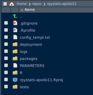
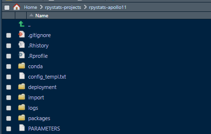
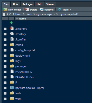
From RStudio, the master project will look like this:

From Windows File Explorer:

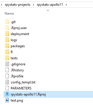
What is new in a RPyStats master project with a typical RStudio project is this:

1. A config_templ.txt file
2. The deployment folder
3. The logs folder
4. The packages folder
5. The PARAMETERS file
6. The conda folder, which you don’t see here yet because we haven’t sent the command to add the Python dependencies.

For the moment there are two objects of interest: the PARAMETERS file and packages folder.

2. Change (cd) to the master project directory

Because we will be sending commands only applicable to this particular project, we have to enter into the rpystats-apollo11 folder.

cd rpystats-apollo11

3. Add a master package

Now that we are in the master project folder, we start creating packages, folder or sub-projects. For this example, we will create the package apollo11.pkg. This package will contain the R and Python libraries definition. You create a child-package with this rsuite command from the terminal:

 rsuite proj pkgadd -n apollo11.pkg

If you enter into the packages folder, you will see this:

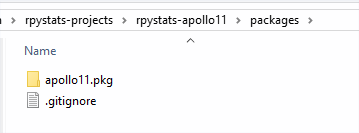
And if you enter into the folder of package apollo1.pkg you will find a typical R package structure, including version control files such as the .git folder. In the next step, we will edit the DESCRIPTION file in the master package.

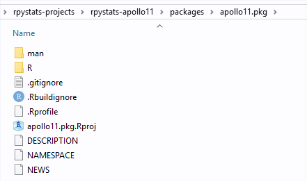
4. Describe the R and Python packages in the DESCRIPTION file

If you are in RStudio, click on the DESCRIPTION file. We want to edit it. This is how the original DESCRIPTION file looks like:

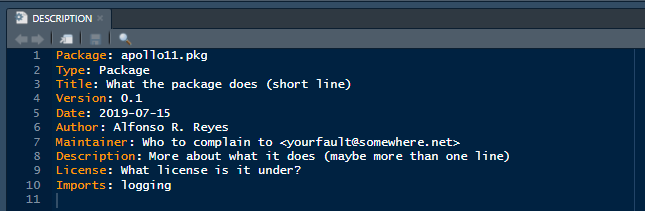
In R, the DESCRIPTION file defines the capabilities of the package. Here we enter the R libraries, and Python libraries, that will be required for the application. After entering these library definitions save the file.

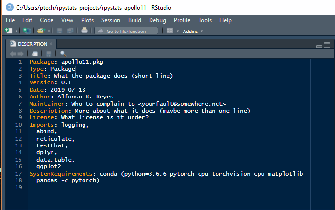
Take a look at the keywords Imports and SystemRequirements.

There are seven R packages that we will use in this project, while in Python we go full machine learning and declare these requirements:

• Python 3.6.6
• pytorch-cpu
• torchvision-cpu
• matplotlib
• pandas

with:

SystemRequirements: conda (python=3.6.6 pytorch-cpu torchvision-cpu 
    
      matplotlib pandas -c pytorch)

The parameter *-c pytorch* indicates the name of the conda packages channel.

In this example, we chose Python 3.6.6 but we could have indicated 3.7 or lower, If our computer has a GPU, we could just change the keyword -cpu. Notice also that numpy has not explicitly been declared because it is automatically installed by PyTorch.

Warning: if you omit the keyword cpu, PyTorch will install the GPU version of the packages. You may get an error if you run Python or R scripts calling the library without your machine having a GPU.

5. Indicate in the PARAMETERS file that Python conda will be used

Now, we go back to the master project and open the PARAMETERS file. We will add the keyword *conda* at the end of the line of Artifacts. Then, save the file.

Artifacts: config_templ.txt, conda

Of course, there are more powerful things you can enable in this file that you can discover by browsing the rsuite tutorials, or see them explained in the next articles.

6. Install the R dependencies

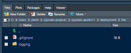
Now, it is the time to install the R packages. After we issue the command the packages that were spelled out in DESCRIPTION, and their dependencies, will be installed. Here is a view of the *deployment/libs* folder before the action taking place:

To start the R packages installation we send this rsuite command:

rsuite proj depsinst

After few minutes, the process ends with an output similar to this:

$ rsuite proj depsinst
2019-07-15 11:02:16 INFO:rsuite:Detecting repositories (for R 3.6)...
2019-07-15 11:02:16 INFO:rsuite:Will look for dependencies in ...
2019-07-15 11:02:16 INFO:rsuite:.          MRAN#1 = https://mran.microsoft.com/snapshot/2019-07-15 (win.binary, source)
2019-07-15 11:02:16 INFO:rsuite:Collecting project dependencies (for R 3.6)...
2019-07-15 11:02:16 INFO:rsuite:Resolving dependencies (for R 3.6)...
2019-07-15 11:02:23 INFO:rsuite:Detected 48 dependencies to install. Installing...
2019-07-15 11:04:58 INFO:rsuite:All dependencies successfully installed.

Forty eight dependencies were installed. Let’s take a look what was installed:

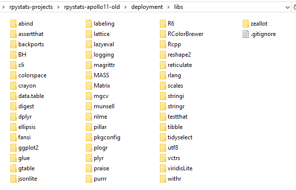
All of these are R packages, the ones we manually indicated in the DESCRIPTION file plus their dependencies.

7. Install the Python dependencies

Now it is Python’s turn. To install the Python requirements we issue this rsuite command:

rsuite sysreqs install

if we explore the folder conda, we will see new folders and files added:

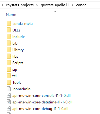
In Windows, the files under the conda folder include python.exe and associated DLL files. Remember, this is a full autonomous Python installation.

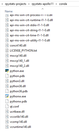
In this step we accomplish two things: (i) install a fully standalone Python installation, and (ii) install the Python libraries we specified in the DESCRIPTION file.

8. Housekeeping

The housekeeping activities will help creating the environment to run the Python and R notebooks, which involves finding and loading the R and Python libraries from any folder under the master project.

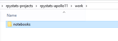
• Add the folder ./work/notebooks for placing the notebooks
• Set the HOME folder in the Windows user environment
• Modify the .Rprofile in the master project
• Add a .Rprofile under the ./work/notebooks folder
• Modify the file ./R/set_env.R

(i) Add the folder ./work/notebooks for placing the notebooks

You can do this from RStudio or from Windows File Explorer. Obtain something like this:

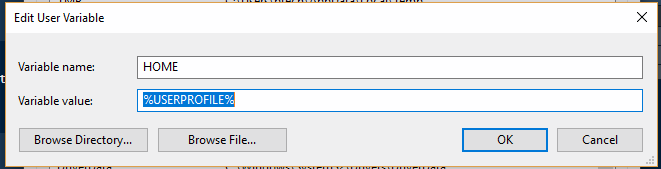
(ii) Set the HOME folder in the Windows user environment

Because we will be using the Unix file system notation in the notebook, we want the home folder (~/) to point to the user directory. We can do this by setting the environment variable HOME to the variable %USERPROFILE%. Like this:

(iii) Modify the .Rprofile in the master project

Copy the code in this GitHub gist to the .Rprofile file located in the master project and save it. You should get this:

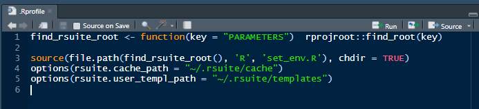
under the master project folder:

(iv) Add a .Rprofile under the ./work/notebooks folder

Copy the code in this GitHub gist to an empty text file named .Rprofile and save it under ./work/notebooks. You should get this:

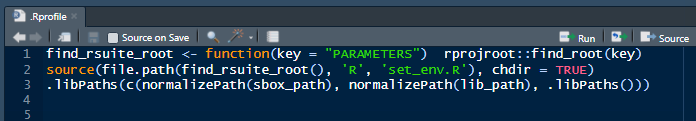
under the folder ./work/notebooks:

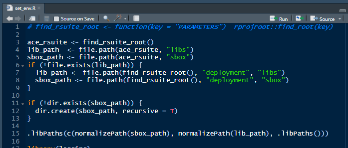
(v) Modify the file ./R/set_env.R

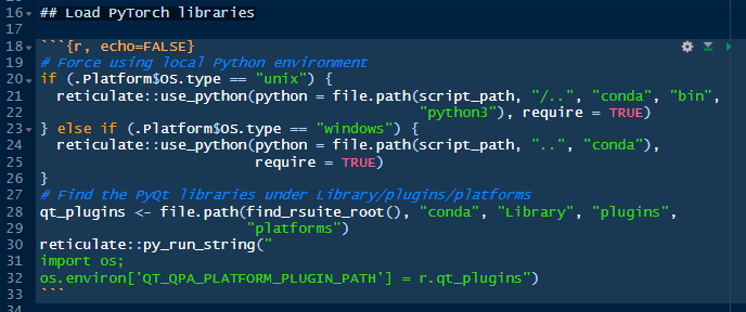
The last housekeeping task is modifying the original set_env.R file under the R folder in the master project. You may not have to do this in other RPyStats projects but because we are using notebooks and it is our first project, we will make it easier. Open the file ./R/set_env.R and replace the code with this GitHub gist. Save it. The first lines of the script would look like this:

9. Add the application code in Rmarkdown notebooks

Okay. At this point we should have the core of the application (executables, packages and libraries) installed. Now, it is time to run some code. This is what we are going to do:

1. Download the MNIST digits dataset and place it somewhere in our master project

2. Create a Rmarkdown notebook for PyTorch experimentation written in Python.

3. Create a second Rmarkdown notebook for PyTorch experimentation written in R.

4. Download the MNIST digits dataset

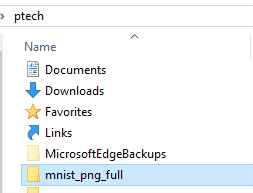
First, download the MNIST digits dataset from here. Unzip the file and copy the contents under the user home directory. In my machine with the Windows user ptech, it would look like this:

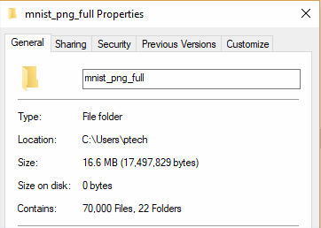
Inside the mnist_png_full:

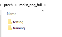
These two folders contain the images, in PNG format, for the training and testing datasets. They have approximately, 16.6 MB of files.

We will show how to load these datasets from the Rmarkdown notebooks in a little bit.

\2. Create the Rmarkdown notebooks in Python

First we will create a notebook with the Python code to run the PyTorch neural network. In you are in RStudio, create a Rmarkdown notebook by clicking on the icon with the plus (+) sign on the left below the menu option File:

You will see a options menu pop up. Click on the second option that reads R Notebook. If you are coming from Python this is the closest to a Jupyter notebook with the major difference that Rmarkdown notebooks are 100% reproducible and capable of version control.

If your RStudio installation is new, or you have never created a notebook, a dialog box will open prompting you to install R packages required to create notebooks.

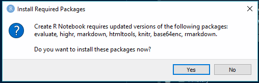
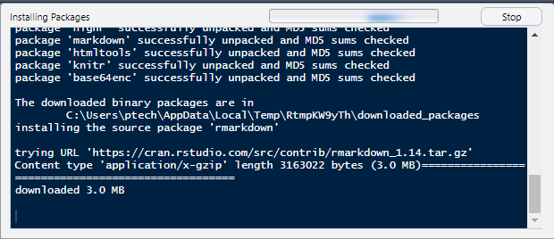
Respond with yes, and the packages installation starts immediately in the background:

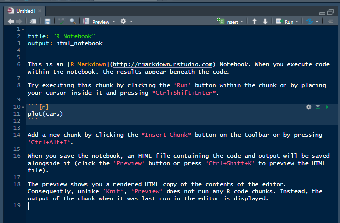
The new notebook opens:

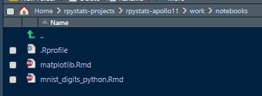
We are going to save the notebooks in a new folder ./work/notebooks. You can create it from RStudio by clicking on “New Folder”:

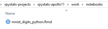
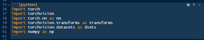
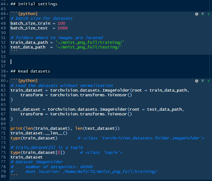
Clear the content in the notebook. Copy the code from the following GitHub gist and paste it in the empty notebook. Save the notebook as “mnist_digits_python” under ./work/notebooks. You should get this structure.

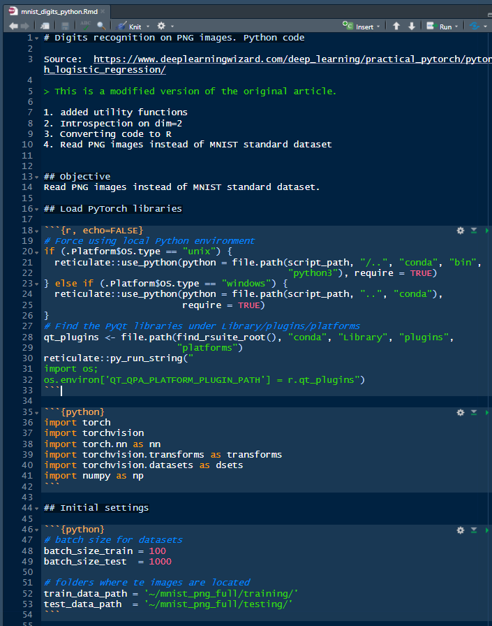
The head of the file would look like this:

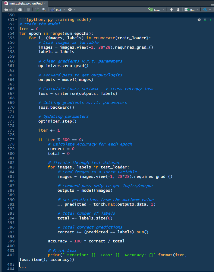
and the tail of the same notebook:

\3. Create the Rmarkdown notebooks in R

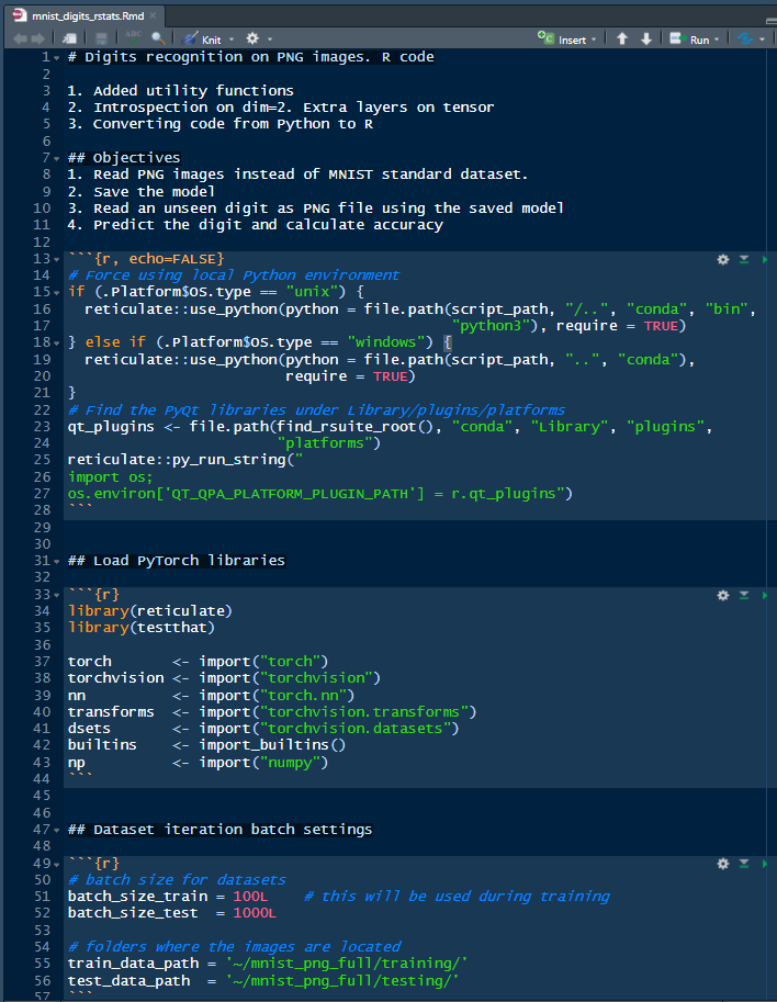
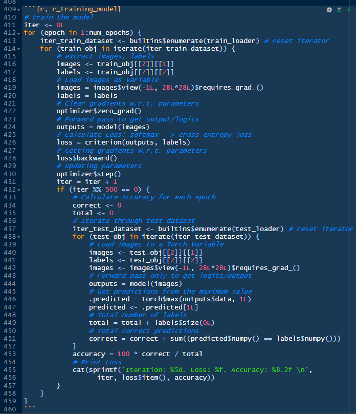
We will proceed similarly with the notebook with PyTorch written in R. Create a notebook, clear the file and copy/paste the following code in this GitHub gist. Save the notebook as *mnist_digits_rstats. R*. This is the head of the notebook:

and the tail of the same file:

We are ready to run these two notebooks.

10. Run the notebooks

There are several ways of running the notebooks. One, run chunk by chunk. Two, run the whole notebook (all chunks) as a session. Three, knit the notebook as a HTML file. And many more.

Let’s start with the Python notebook executing the code chunk-by-chunk.

Note that each code chunk in the notebook has three symbols on the top right corner. We are interested in the green arrow, which means “run this chunk”.

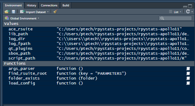
Some of the chunks will show output some others won’t. It depends if you defined it to do so. The particular chunk at the top (picture above), will not show any output but you will be able to see some activity on the Environment pane in RStudio.

Move to the second chunk and run it by clicking on the green arrow. If you copied correctly the .Rprofile and modified the file set_env.R, there will no errors.

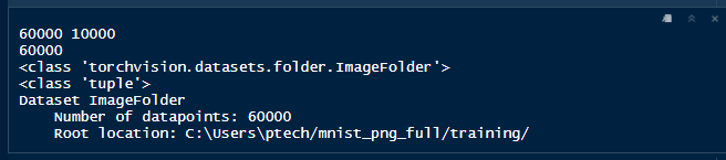
Then the third and the fourth:

Now we start getting output. What this is showing is the size of the training set (60,000 images); the size of the testing dataset (10,000 images); the class of the object train_dataset; the type of the Python object; and the informative string of the train_dataset object.

Continue executing the chunks while reading the comments to understand what each block of code does. That is the wonderful thing about notebooks.

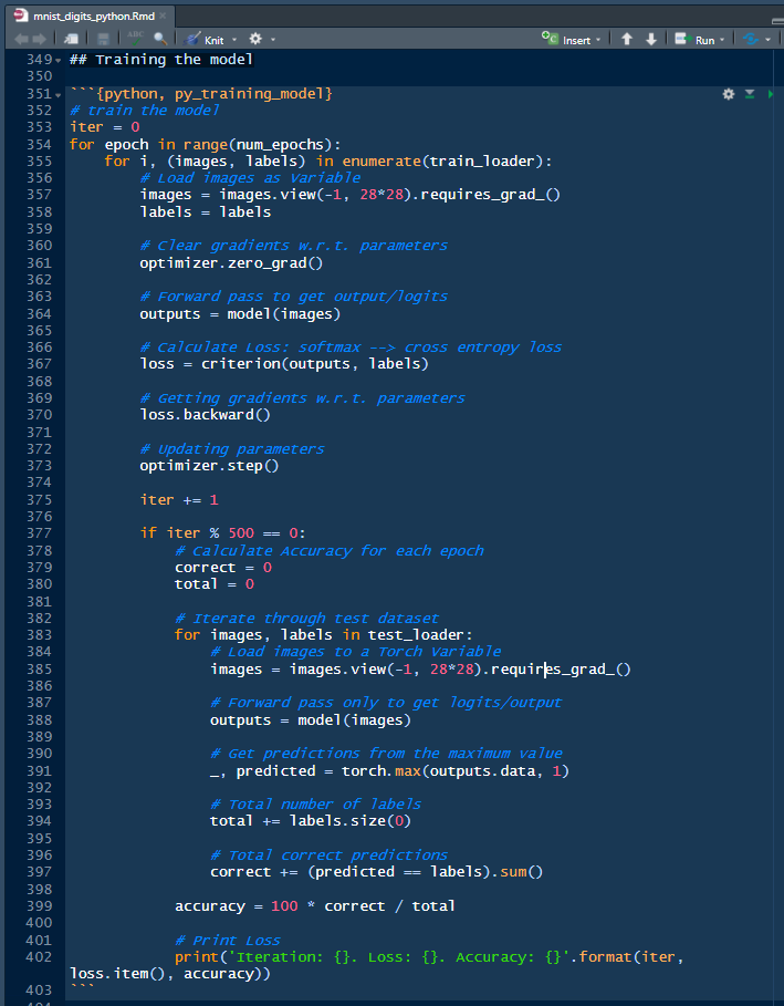
Continue running the chunk until line 350. The following chunk will perform the training on the dataset, and at the end of each epoch will calculate the accuracy on never-seen samples, or testing dataset.

After you click on the run arrow, it will take about five minutes to complete the training. This is the output that we were looking for:

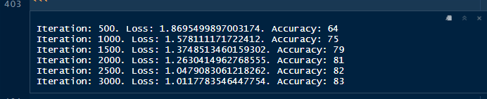
It is a good accuracy given the fact that we didn’t touch the data or perform any normalization, etc., nor applied a complicated algorithm. Only a simple logistic regression. Later in the episodes, we will change the algorithm to a neural network.

In the next episode, we will run the PyTorch code notebook but totally written in R.

Example repository

[https://github.com/f0nzie/rpystats-apollo11](http://Example repository https://github.com/f0nzie/rpystats-apollo11)

Links

• MNIST digits dataset: https://github.com/f0nzie/mnist_digits_png_full
• .Rprofile gist to save in master project: https://gist.github.com/f0nzie/82d056541227d569029be7b7787fbb24
• .Rprofile gist to save in ./work/notebooks: https://gist.github.com/f0nzie/0493dc541f68903584d22ce6179dab23
• Script gist set_env.R in the R folder: https://gist.github.com/f0nzie/0fff8c5ec57b2ffc49ed177d770cc9c3
• Rmarkdown notebook with PyTorch Python: https://gist.github.com/f0nzie/90749827f43583638b5c9cf382424f9b
• Rmarkdown notebook with PyTorch R: https://gist.github.com/f0nzie/9a2e798e474bcee3c6e60acdeb34876f