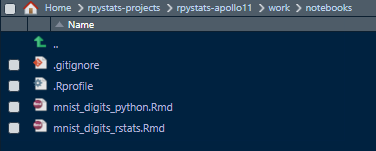
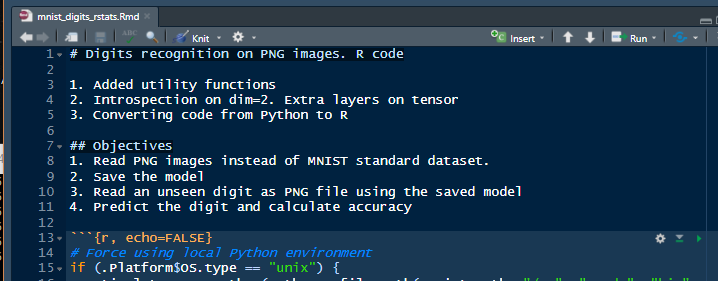
In the previous episode we ended up calculating the accuracies for the MNIST digits model using PyTorch libraries called from a Rmarkdown notebook written in Python. In this episode, we will run the same example but in another notebook written in R named *mnist_digits_rstats.Rmd*, which was saved in the folder ./work/notebooks in the previous session. With RStudio open, let’s click on the file to open it.
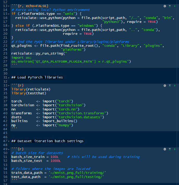
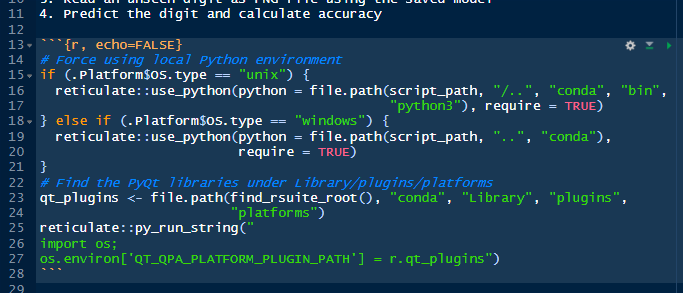
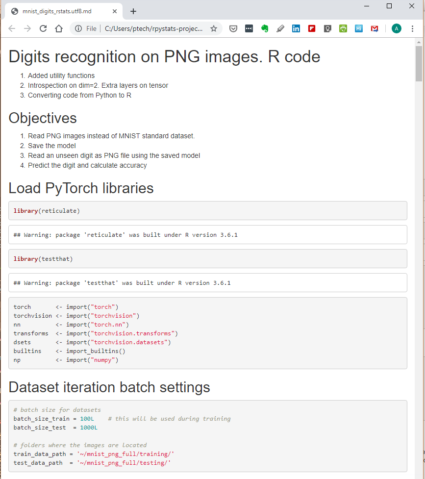
You may notice some familiarity between the code in this notebook *mnist_digits_rstats.Rmd*, written in R:
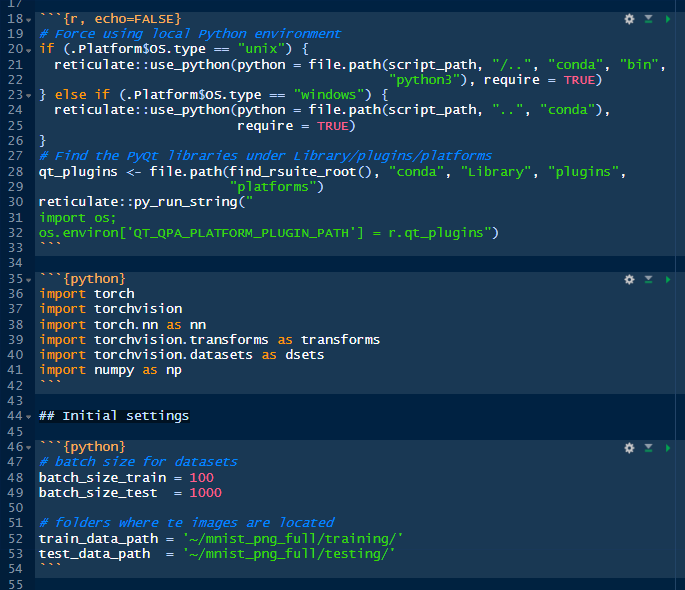
versus this other code in the first notebook *mnist_digits_python.Rmd,* that we have already run, written in Python:
Both look familiar but they are not the same. Each language uses it own syntax and conventions that makes them unique and powerful. We will explain the details later. For now, we are interested in running the notebook in R.
Running the notebook in R or Python show similar characteristics. Since we are still exploring let’s continue running individual code chunks by clicking in the green arrow on the first block:
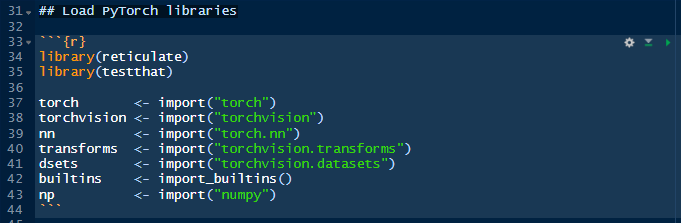
Then, the second chunk that loads the PyTorch libraries, numpy and Python built-in functions:
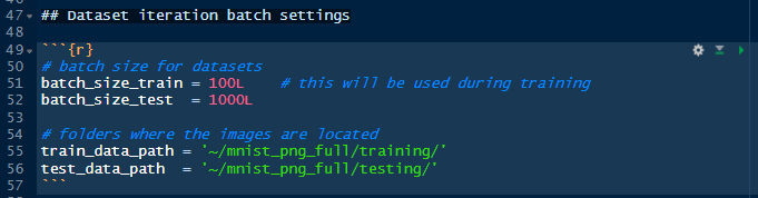
We don’t get any output in response because we haven’t explicitly ordered the script to do it. Then, we run the next chunk of code where we indicate the size of the training and testing batches, and the location of the training and testing datasets on disk. Note that the location of the datasets is the user home directory under the folder *~/mnist_png_full/*
After runnig the chunk, still we get no output because we are just assigning values to objects.
Now, it’s the turn of the fourth block, which will load the raw images from the training and testing datasets and assign them to two objects: train_dataset and test_dataset.
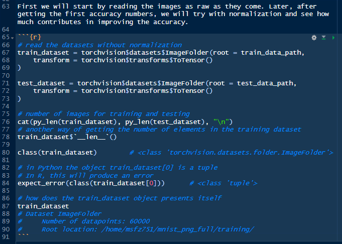
This time we get some output, which is informative about the number of images in the training and testing datasets, besides class and type of the objects being loaded, additionally to the description of the object *train_dataset*.
Continue running the individual chunks while observing the output and the comments of what that code does. Stop at line 325. We will pause to take a look at a piece of code.
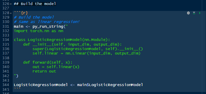
The following chunk will serve us very well because it represents the confluence of Python and R. The class that is being defined here is named *LogisticRegressionModel*. This is the algorithm that will be used to train the model. This class is inheriting from another class: Linear, which is part of the torch.nn library. We will just add a method to the class, forward(), before we finish. What it is interesting here is that the machine learning class is entirely written in Python, not in R. I will not explain now why is has to be that way in this episode. The class (code in green), is then assigned to the *main* object in R, and immediately extracted from main itself, to an R object named *LogisticRegressionModel*, same as its relative in Python. Note that we used the dollar sign *$* to extract an object from main. This *$* sign is how you extract objects in R, while in Python we use the dot, like in *nn.Linear*.

This block doesn’t print anything but the next one will. Move your cursor to the next chunk, press on the green arrow. And you will get an output.
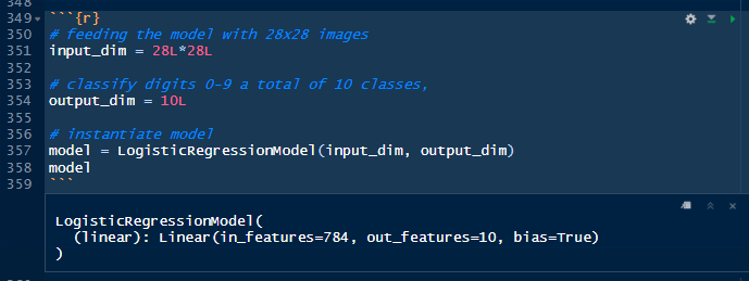
Besides indicating the size of the input and output, we are printing the settings of the class *LogisticRegressionModel*, which is confirming for us that the number of features in the input is 784 (number of pixels in a 28 by 28 matrix), and features in the output is 10 (number of digits from 0-9).
In fact, we are scratching the surface in terms of learning more about the internals of Python and its interaction with R. We are skipping lot of material for now. But you could learn a lot now just by comparing the notebooks in Python and R, chunk by chunk.
Our next stop, before closing this episode, is moving the cursor to the last chunk in line 409. Everything that has been prepared, defined, and set here has been with purpose of making the following loops to work: The epoch loop; the training dataset loop; and the testing dataset loop.
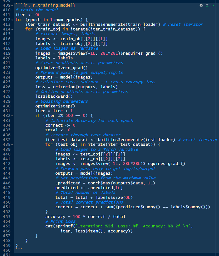
The loop we are most interested in is the one in the middle because it iterates throughout all the 60,000 hand-written digit images to learn.
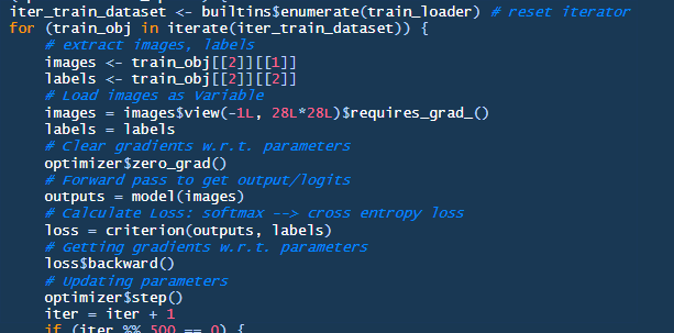
You will find that the code in R in this chunk is pretty similar to its counterpart in Python. The difference is primarily how we address the objects, such as the iterator train_loader, iter_train_dataset, and train_obj. Everything else is pure PyTorch with R notation.
The other loop that is interesting is the inner loop, which calculates the accuracy after the training dataset went through an epoch.
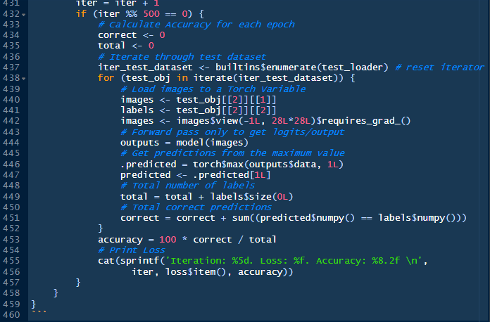
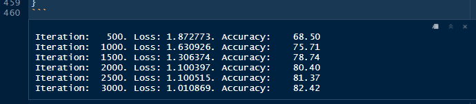
The iteration on the testing dataset and addressing the objects is similar to the loop above. But this time we are calculating how many of the predicted images from the training job are matching the unseen digit images in the test dataset, and then calculate the percentage of correct predictions respect to the total number of images in the test dataset. This calculation is performed at the end of every epoch. There are five epochs.
If we run the chunk it will take few minutes and give us this output, which is pretty approximate to the results given by the Python Rmarkdown notebook.
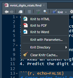
One more thing we are going to do before closing this episode is printing the notebook to a HTML file or web page that you can view in a browser. To do this we will move our attention to the top part of the pane. Just below, to the right of the name of the notebook, there is a little blue icon with the label Knit.
Click on the little down arrow and you will see this menu pop up. Select the first option “Knit to HTML”. Let’s give a few minutes to R to perform the calculations and compile the notebook.
After 3 minutes - the time approximately takes to run the algorithm, you will get this window which is the RStudio built-in browser. Click on the button that says “Open in Browser”.
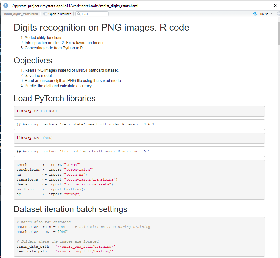
Now, the page with the results will open in a new window in the default browser, giving you the possibility of immediately sharing your work via the web.
There many more possibilities for publication, which is one the strongest points of R and RStudio. You could print to a PDF, to a Latex or TeX file, to a Word file, or to a set of slides with choice of various formats, including PowerPoint. The Rmarkdown notebook has extraordinary powers which do not end with the calculations in cells or chunks but expand to plenty of output formats. That one of the greatest advantages of using RPyStats.