Building your petroleum engineering library with R: Muskat's Material Balance Equation ODE

ODE Solvers

In the ODE solvers that are part of the package rODE, the differential equation is entered as an object and then placed inside a loop where the iterations takes place. The number of steps and the size of the steps can be chosen by the user, as well as the state variables. That includes the selection of the ODE solver. At this moment I have implemented these solvers in R:

• Euler
• Euler-Richardson
• Verlet
• Runge-Kutta, RK4
• Dormand-Prince, or RK45, with an adaptive step

It is not necessary to tell you which one is the best. You will be able to find out by yourself. There are nine articles or vignettes in the rODE package website that will guide through the construction of your differential equations.

What’s rODE

This is not your typical black-box ODE solver. With rODE, you really have to develop your ODE algorithm using any of the ODE solvers available. The objective is learning R while coding, understanding the physics of petroleum engineering, developing algorithms and applying math.

rODE was my first R package that I developed to really understand the power of R, how a package is made, the principles of functional programming, and the use of object orientation with S4 classes. R has not one but several ways of achieving object orientation: S3 classes, S4 classes, R6, Reference classes, and I believe, a couple more. I kid you not. You will never run out of gas.

Muskat’s Material Balance Equation

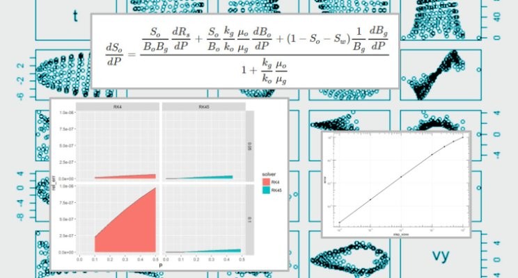
Going back to the main topic of this article: Muskat’s Material Balance Equation, I use it as an example of the ODE solver. I know, it is a basic example, but great to start getting your hands wet with some ODE solvers. Here is the equation:

# equation

Since all the terms on the right side are function of pressure (P) and saturation (S), the equation could be reduced to dS/dP = f(P, S). The equation on the left look ugly because LinkedIn does not support Latex equations or markdown yet. That’s why I am giving you here the link to the rODE website, so could see the real thing. Click here. That link will bring directly you to the vignette on Muskat’s Material Balance equation solved with rODE. Explained step by step.

What’s the goal

The objective is solving the equation using all ODE solvers available and show the relative error between the solver solution and the analytical solution, which we are calling here the exact solution. The idea is that you decide what is the more accurate and efficient ODE solver for your problem. Since in the example we know in advance the analytical solution -which in most of the cases we don’t -, we will add a method getExactSolution to return the exact values at any given pressure P. Then we will compare the exact solution versus the numerical solutions from the available ODE solvers in rODE. Here is the code where the Muskat’s differential equation is entered. We call this class MuskatODE.

# code

One word of advice: do not feel intimidated by the code here. It will become rapidly natural to you in few sessions of R. And remember, R is not only an amazing tool for engineering but for data science, machine learning and neural networks.

Data Science is to today what the PC was in the 80’s, or early 90’s

Control of the ODE solver

After we define the differential equation in shape of code, or ODE object, we move to build the iterative routine for the differential equation. We start with the given initial conditions, P=0, and S=1, stopping the iterations at P=0.5. Don’t mind for now the units.

This is the part where all the interesting things happens: the solver control loop.

# code

The function MuskatEulerApp only receives the size of the step and the while-loop will stop until reaching a maximum pressure of 0.5.

After the iteration model is completed, it is time to analyze the results stored in the table. We do this by sending the three step sizes for ΔP using the function lapply.

# code

Since we don’t want to see all the intermediate steps, we will limit the result table to display only the solutions at P equal 0.10, 0.20, 0.30, 0.40, 0.5.

# code

Table with ODE solver results

The table has these columns or variables:

• step_size: size of the step for the solver.
• P: pressure
• S: saturation
• exact: exact value from the analytical solution
• error: difference between the analytical solution and the numerical solution
• rel_err: relative error
• steps: number of steps taken by the solver

This is the code that we use to generate all the tables for the steps 0.2, 0.1 and 0.05.

# code

That little bit there with lapply is just the tip of the iceberg in functional programming. And there is a lot of it in R. Say bye-bye to the for loops!

And this is the first table with results:

# code

We can see from the table that for the smaller step size of 0.05 at P=0.5, we get a relative error of approximately 0.0306, or 3%. We will improve this by using more efficient solvers.

Functional programming: two nested lapply functions

Since all the steps look much better in the rODE website, I will just jump fast forward to the interesting part. Generating, with few lines of code, a rich summary of the relative errors for all the steps for all the available solvers. These are the input vectors:

# code

And these are two nested lapply functions:

# code

The resulting table (I am cutting few values to make it fit here in LinkedIn):

# table

Tidy tables

This is almost a tidy table! Why almost? Because the saturation column S and the exact columns should be grouped together in one column; let’s call it saturation, and an additional column should tell us if the value is of type “solver” or “exact”. By transforming your table in tidy format you enable even more powerful plots.

Plots of errors vs ODE solvers

And the plot showing the errors for each step and every ODE solver.

# plot

In this last plot we want to compare the relative error of the ODE solvers that show the least error: RK4 and RK45. At the same time, we will exclude the step size of 0.2 since its error magnitude would hide those of the smaller steps.

# plot

It turns out that RK45 is the more accurate of all the solvers tested here. The relative error at a step value of 0.05 is in the order of 1E-8 to 1 E-12, while RK4 for the same step size, the relative error ranges between 1E-8 to 9E-8; still good. In fact, we could choose with some peace of mind RK4, unless the response is so unstable that merits the switch to an adaptive step solver such as RK45. RK4 is widely used by its balance of accuracy and computational speed.

Please, visit the rODE website for a detailed expanation of the solution. Also have access to other eight examples.

As always, all the code, notebooks, datasets, plots. references are available at GitHub at this repository.

Breaking News

rODE v0.99.6 has been approved by CRAN and available to install from the CRAN repositories.

Follow me in Twitter: fonzie@OilGains

References

The following books and papers were consulted during the development of this package:

[1] R. Ashino, M. Nagase and R. Vaillancourt. “Behind and beyond the Matlab ODE suite”. In: Computers & Mathematics with Applications 40.4-5 (Aug. 2000), pp. 491-512. DOI: 10.1016/s0898-1221(00)00175-9.

[2] K. Atkinson, W. Han and D. E. Stewart. Numerical Solution of Ordinary Differential Equations. Wiley, 2009. ISBN: 978-0-470-04294-6.

[3] J. R. Dormand and P. J. Prince. “A family of embedded Runge-Kutta formulae”. In: Journal of computational and applied mathematics 6.1 (Mar. 1980), pp. 19-26. DOI: 10.1016/0771-050x(80)90013-3.

[4] H. Gould, J. Tobochnik and W. Christian. An Introduction to Computer Simulation Methods: Applications To Physical Systems. CreateSpace Independent Publishing Platform, 2017. ISBN: 978-1974427475.

[5] T. Kimura. “On dormand-prince method”. In: Retrieved April 27 (2009), p. 2014. <URL: http://depa.fquim.unam.mx/amyd/archivero/DormandPrince_19856.pdf>.

[6] M. A. Nobles. Using the Computer to Solve Petroleum Engineering Problems. Gulf Publishing Co, 1974. ISBN: 978-0872018860.

[7] T. Ritschel. “Numerical Methods For Solution of Dierential Equations”. Cand. thesis. DTU supervisor: John Bagterp Jørgensen, jbjo@dtu.dk, DTU Compute. Technical University of Denmark, Department of Applied Mathematics and Computer Science, 2013, p. 224. <URL: http://www.compute.dtu.dk/English.aspx>.

[8] R. Sincovec. “Numerical Reservoir Simulation Using an Ordinary-Differential-Equations Integrator”. In: Society of Petroleum Engineers Journal 15.03 (Jun. 1975), pp. 255-264. DOI: 10.2118/5104-pa.

[9] K. Soetaert, T. Petzoldt and R. W. Setzer. “Solving differential equations in R: package deSolve”. In: Journal of Statistical Software 33 (2010).