Few weeks ago I was working on the marching algorithm to create vertical lift performance (VLP) curves and datasets for statistical analysis using the classical Hagedorn-Brown and Fancher-Brown correlations. Then I noticed some weird variations in the column for the compressibility factor or z. I started to investigate and found discontinuities in parts of the isotherms that are used for building the gas compressibility correlations. Digging a little bit more finally found that the problem was that the values of the fluid properties of my well had accidentally hit a critical point in the equations. What is the chance?
Though it was no my intention on working on the compressibility factor z for hydrocarbon gases, the issue opened my curiosity; now I wanted to know more about the gas compressibility equations and take a look at the origin of these discontinuities. After reading a few papers, couple of books and a thesis on the subject (see citations at the bottom), I feel now more confident about the range of applicability of the different compressibility correlations. And R is the perfect partner for that analysis. You will find out why later.
I will not go too much in detail in this article because it is very well explained with the package in GitHub (see link at the bottom), which includes several notebooks or vignettes showing each of the correlations step-by-step, as well as instructing how to use the functions. You will find this documentation as well as the code, functions, notebooks, plots, citations in the package zFactor itself.
I highly recommend you do something different and daring today and install R and RStudio and experiment yourself.
Correlations for compressibility I decided to focus on the sweet gases first, since they are simpler to deal with and they not require additional corrections as the sour gases do. These are the correlations I analyzed:
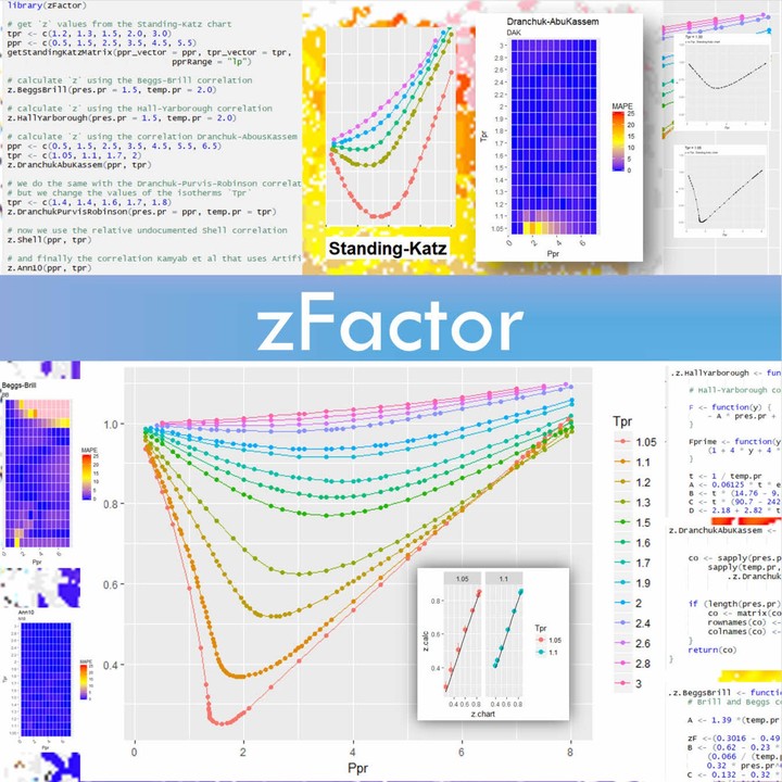
Beggs and Brill (BB) Hall and Yarborough (HY) Dranchuk and Abou-Kassem (DAK) Dranchuk, Purvis and Robinson (DPR) A correlation by Shell Oil Company (SH) A correlation developed with Artificial Neural Networks (Ann10) by Kamyab et al (N10) The figure below rapidly summarizes the findings of the work. MAPE is the Mean Absolute Percentage Error and is shown as the gradient bar on the right: blueish is very low error; reddish is bad, near 25% deviation from the Standing-Katz (SK) chart baseline; pink is above 25%. What do you think? I know, I know. You are curious about the correlation Ann10, right?
My baseline was going to be the Standing-Katz (SK) chart. For the comparison I used two approaches to better understand z in the chart: creating a table (dataframe) of errors or deviation of z (calculated) from the SK chart, and a plot where we could see the areas of the pseudo-reduced pressure (Ppr) vs. pseudo-reduced temperatures (Tpr) that were holding more error. The numerical and graphing visual paints a clearer picture of what the authors of the correlations were trying to convey. It is not a simple “Tpr works from to here to there, or Ppr should be in this range”. That’s too general a statement. What about seeing or testing for ourselves? And regarding this point of the range of applicability of the correlations, I found contradictions, not only in the papers, but in the reality of the calculation results.
The Standing-Katz chart The work starts by digitizing the Standing-Katz chart. If you recall from college at your reservoir and production classes is that awesome chart produced in 1942 by these pioneers Marshal B. Standing and Donald L. Katz. It was a set of pseudo-reduced temperature curves (Tpr) or isotherms, with one the sharpest resembling a “v” (Tpr at 1.05) versus pseudo-reduced pressures on the x-axis with a grid at 0.1 steps. The compressibility factor ‘z’ appears on the y-axis.
Any of the researchers and correlation authors had to go through the same ordeal of digitizing the curves in order to establish a baseline for performing the comparison of the equation calculations versus experimental data. I looked up in the internet and some universities and I could not find a dataset of the SK chart. In some of the curves taking a value of z every Ppr=0.5 seems to be enough, specially in the regions where the curves are linear. In other regions, you will see that is necessary to take at 0.1 in the Ppr axis or even less. You will be able to see the raw data of the digitized Standing-Katz chart in text files under inst/extdata.
Once that is done, these curves can be immediately plotted or statistically analyzed using R functions. I have added several function for plotting, creating tables, matrices and dataframes from the SK chart as well from the results from the correlations.
A sample of an equation for finding gas compressibility Just to show you a quick example, you will see below the R code for the algorithm that calculates z using the Dranchunk-AbouKassem method. Neat and simple. The rest of the code for the other equations (Hall-Yarborough, Dranchuk-Purvis-Robinson, Shell and Neural-Networks-10), can be found in GitHub. All of them receive as input the pseudo-reduced pressure and temperature. This can be, of course, enhanced to receive as inputs the pressure and temperatures at depth, and if the proper corrections are made, the percentages of CO2, H2S and N2.
Why “R” is intermingled with reproducibility Since I am all for reproducibility of any scientific or engineering work, I am making the code, the equations, the algorithms, the plot generation, the paper citations, all available in GitHub so you could download it and reproduce this work yourself. Here is the link: https://github.com/f0nzie/zFactor. Or you just install it from CRAN, the R repository. You will need first to install R (it’s free). I use RStudio (also free) on top of it to make a faster development. You will see that working with R is delightful, fun and fulfilling because it always works. The standard for software publication, what they call packages, is very high.
A petroleum engineering library with “R” Why do I mean by this? Once you start developing your own functions, not in Excel VBA or macros, but the same work in R, you will see that the knowledge value starts to grow. And I am not talking only about the code sharing. I mean the data originated by the models in the shape of datasets. That’s what makes data science unique to petroleum engineering: add value, perpetuate the knowledge, document the findings, improve the quality, start the discussion, find the answers and explain the solution.
Your petroleum engineering library is customized to your specific challenges and could be including topics like reservoir engineering, reserves estimation, gas lift optimization, well testing, nodal analysis, sucker rod pump analysis, ESP diagnostics and optimization, sand control, fracture post-analysis, completion design selection, flowing and static gradient history, IPR and VLP curves profiling, and dozens of other applications.
The value to an E&P company -of any size or complexity-, comes from different fronts: a stable engineering platform that runs under all operating systems, infinite plotting capabilities, unique statistical base, intuitive solutions, knowledge preservation, diminishing license issues, ownership and integration. And last, and more importantly, preparing your team for machine learning and artificial intelligence development.
You can follow me via Twitter via fonzie@OilGains
The code, documentation and instructions are available at: zFactor at GitHub