Introduction
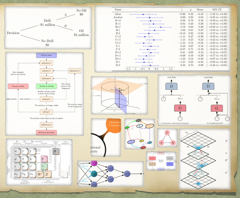
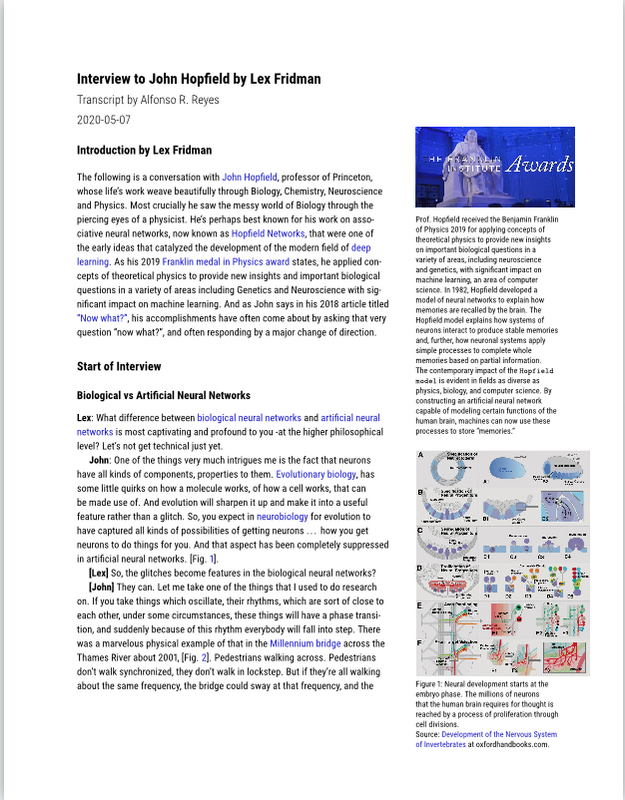
I have been working a lot lately with LaTeX and TikZ graphics. I am preparing a paper and few articles that need some sketches and wasn’t able to find the right tool to do it. I am a markdown guy and almost everything I write is either in Markdown or Rmarkdown files. One of the last documents I wrote using Rmardown was the transcript of the interview to Professor John Hopfield. The ideal type of document was a Tufte style article to include context on the margins, graphics and sidenotes. A screenshot of the first page below.
During my TikZ “training” and learning experience I collected quite a few TikZ source files. I like them because they facilitate learning the TikZ language. If we can call it that. The problem with accumulating source files over time is that you lose track of them -there is not a viable way to organize and extract value of information just by using the operating system file explorer.
As a result of that, I found the ideal way is creating a static web site of images (using Hugo), source code and metadata. The sort of site where you click on the image you see the code that generates it. You will read more about that in a minute.
What is TikZ
TikZ is ideal for any kind of publications either websites, blogs, papers, articles, slides, or books because they are portable and reproducible. TikZ files are text not binary files. They don’t require mouse and clicks but writing code to connect objects and elements. These objects can be very simple or as sophisticated as you want. TikZ graphics can be built under any LaTex environment that installs under any operating system: Windows, Linux or Mac OS.
There are hundreds of libraries for TikZ that cover practically all scientific fields. That makes it easier to build advanced graphics for practically any domain or discipline because you are able to start from code already written.
Motivation
While working with LaTex and TikZ files I had this question:
How can I use the power of R to organize TikZ related files?
R is very friendly to LaTex and TikZ through the packages knitr and Rmarkdown.
TikZ involves a source file, which carries the “tex” extension; the PDF that is generated by your Latex compiler and editor (I use TexStudio); and the graphics output file -that could be any format imaginable. I use “png” files.
Results
There are two main outcomes from using R to tackle this file organization problem:
- A static website generator that builds an index.html with all the links to the graphics (.png) and code (.tex) living in your source folder
- An auto-generated README.Rmd that inserts all the graphics and code inside the document
Think of them as: (1) an online gallery of graphics (website) for the former, and (2) a catalog of graphics and code that you can export or view as an Html file or a PDF file from your RStudio IDE.
For starters, I build my first collection of TikZ favorites, generated the static website and published it as a GitHub repository. They are some of the best TikZ examples I have found around the web and from papers, slides, tutorials, and books. Most of the examples are simple enough to encourage anyone to start learning TikZ. By having the result (graphic) on a web page, and be able to click on it to see the code, it rapidly helps to make the connection between code and output. I find this idea fantastic. The website looks like this:
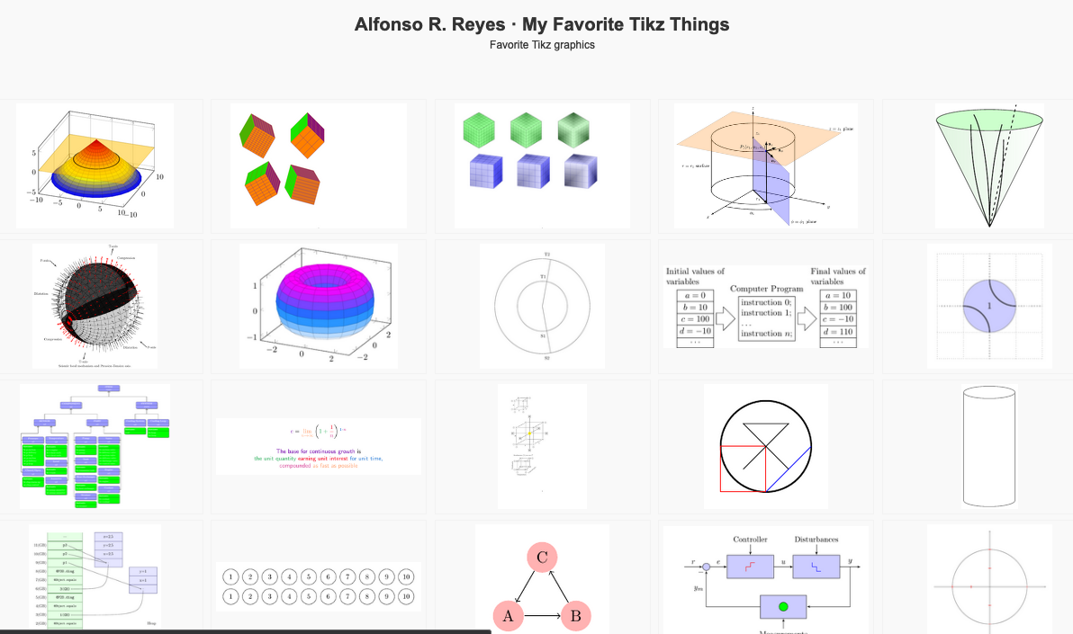
The link to the static website is https://f0nzie.github.io/tikz_favorites/.
I am making use of GitHub Pages to publish the website. That’s why you see a folder named “docs”. The index.html file in that folder contains all the links to TikZ graphics (.png) and the source files (.tex) that are located under the “src” folder.
The GitHub repository looks like any other GitHub repo:
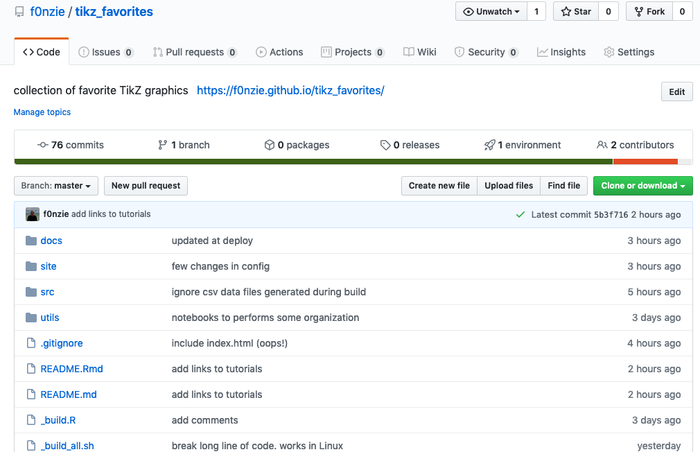
The link is https://f0nzie.github.io/tikz_favorites/
The only difference with other READMEs is that because this README.md has been generated with R code and a Rmarkdown template, it contains all the TikZ graphics and code that live in the source folder “src”. This is all automatic by means of scripts. Scroll down the README in the repo to see.
Since this README is smartly generated with TikZ graphics and code located in the “src” folder, this means that as you continue adding, building, designing new TikZ drawings, they become available to be automatically included in the README in the next build. It uses some knitr tricks. But the whole thing is awesome.
Examples
You may be asking. How does the TikZ code looks like to generate a simple graphic?
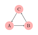
Example 1. I will use a simple example. For this code:
% elem-3_nodes_triangle+elem+foreach.tex
% from Helmund slides
\documentclass[tikz,border=10pt]{standalone}

%\documentclass[crop, tikz]{standalone}
\usepackage{tikz}


\begin{document}

\begin{tikzpicture}[scale=.9, transform shape]

    \tikzstyle{every node} = [circle, fill=red!30]
    \node (a) at (0, 0) {A};
    \node (b) at +(0: 1.5) {B};
    \node (c) at +(60: 1.5) {C};
    \foreach \from / \to in {a/b, b/c, c/a}
    \draw [->] (\from) -- (\to);

\end{tikzpicture}


\end{document}
we will get this graphic:
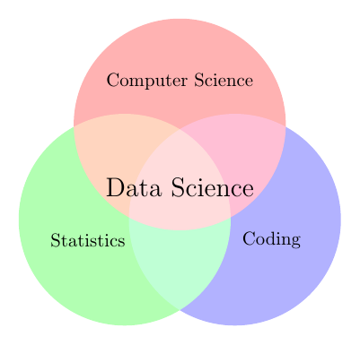
Example 2. You probably have seen this one around.
% impact-venn+diagram.tex
% http://www.texample.net/media/tikz/examples/TEX/venn.tex
% A Venn diagram with PDF blending
% Author: Stefan Kottwitz
% https://www.packtpub.com/hardware-and-creative/latex-cookbook
\documentclass[border=10pt]{standalone}
\usepackage{verbatim}
\usepackage{tikz}

\begin{document}

\begin{tikzpicture}

    \begin{scope}[blend group = soft light]
      \fill[red!30!white] ( 90:1.2) circle (2);
      \fill[green!30!white] (210:1.2) circle (2);
      \fill[blue!30!white] (330:1.2) circle (2);
    \end{scope}
    \node at ( 90:2) {Computer Science};
    \node at ( 210:2) {Statistics};
    \node at ( 330:2) {Coding};
    \node [font=\Large] {Data Science};

\end{tikzpicture}

\end{document}
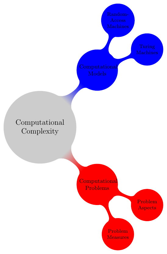
Example 3. The classical mindmap has this simple code:
% mind_optional_argument+mindmap.tex
\documentclass[margin=2mm]{standalone}

\usepackage{tikz}
\usetikzlibrary{mindmap}

\begin{document}

\begin{tikzpicture}[
    mindmap,
    every node/.style=concept,
    concept color=black!20,
    grow cyclic,
    level 1/.append style={level distance=4.5cm,sibling angle=90},
    level 2/.append style={level distance=3cm,sibling angle=45}
    ]
    \node [root concept] {Computational Complexity} % root
    child [concept color=red] { node {Computational Problems}
    child { node {Problem Measures} }
    child { node {Problem Aspects} }
    }
    child [concept color=blue] { node {Computational Models}
    child { node {Turing Machines} }
    child { node {Random-Access Machines} }
    };

\end{tikzpicture}

\end{document}
which yields this output:
I hope you enjoy this article!