Introduction
I recently finished double-converting, from Python to R, and from PyTorch to rTorch, a very powerful script that creates synthetic datasets from real datasets.
Synthetic datasets are based on real data but altered enough to keep the privacy, confidentiality or anonymity, of the original data. Since synthetic datasets conserve the original statistical characteristics of the real data, this could represent a breakthrough in petroleum engineering for sharing data, as the oil and gas industry is well known for the secrecy of its data.
Procedure
I will start by sharing the original code in Python+PyTorch, and immediately below it, the R+rTorch converted code. I will also include some plots of the distributions of the synthetic datasets, as well as numeric results.
This is the link to GitHub repository where I have put the R and Python: https://github.com/f0nzie/gan-rsuite. It consists mainly of Rmarkdown notebooks, a few Jupyter notebooks, a handful of Python scripts with PyTorch, and few other R scripts. The Rmarkdown notebooks explain the conversion and transition from PyTorch to rTorch. So, if you want to learn PyTorch at the same you learn R, this is your chance.
The Rmarkdown notebooks have been numbered in such a way you could follow the transition by the ascending number of the documents.
The plan is explaining a little bit how this algorithm works, the steps to build one yourself in Python or R, show the original dataset, compare it with the synthetic, make some observations from the data artificially generated, and draw some conclusions about sharing synthetic datasets.
GAN in PyTorch
I don’t expect the code to look beautiful here. If you don’t like how the code looks here in LinkedIn, please, visit the repository to take a look. This is the original code as was presented by its author Dev Nag in Medium. I will use this code as a base because it works and is very straight forward and short. The final code will have some minor variations for the output of the GAN metrics and the synthetic data. The code corresponding to this script can be found as “gan_torch.py” under the folder notebooks.
# Generative Adversarial Networks (GAN) example in PyTorch. Tested with PyTorch 0.4.1, Python 3.6.7 (Nov 2018)
# See related blog post at https://medium.com/@devnag/generative-adversarial-networks-gans-in-50-lines-of-code-pytorch-e81b79659e3f#.sch4xgsa9

import numpy as np
import time
import torch
import torch.nn as nn
import torch.optim as optim
from torch.autograd import Variable

matplotlib_is_available = True
try:
    from matplotlib import pyplot as plt
except ImportError:
    print("Will skip plotting; matplotlib is not available.")
    matplotlib_is_available = False

torch.manual_seed(123)
np.random.seed(seed=123)

# Data params
data_mean = 4
data_stddev = 1.25

# ### Uncomment only one of these to define what data is actually sent to the Discriminator
# (name, preprocess, d_input_func) = ("Raw data", lambda data: data, lambda x: x)
# (name, preprocess, d_input_func) = ("Data and variances", lambda data: decorate_with_diffs(data, 2.0), lambda x: x * 2)
# (name, preprocess, d_input_func) = ("Data and diffs", lambda data: decorate_with_diffs(data, 1.0), lambda x: x * 2)
(name, preprocess, d_input_func) = ("Only 4 moments", lambda data: get_moments(data), lambda x: 4)

print("Using data [%s]" % (name))

# ##### DATA: Target data and generator input data


def get_distribution_sampler(mu, sigma):
    # Bell curve
    return lambda n: torch.Tensor(np.random.normal(mu, sigma, (1, n)))  # Gaussian


def get_generator_input_sampler():
    return lambda m, n: torch.rand(m, n)   # Uniform-dist data into generator, _NOT_ Gaussian


# ##### MODELS: Generator model and discriminator model


class Generator(nn.Module):
    # Two hidden layers
    # Three linear maps
    def __init__(self, input_size, hidden_size, output_size, f):
        super(Generator, self).__init__()
        self.map1 = nn.Linear(input_size, hidden_size)
        self.map2 = nn.Linear(hidden_size, hidden_size)
        self.map3 = nn.Linear(hidden_size, output_size)
        self.f = f

    def forward(self, x):
        x = self.map1(x)
        x = self.f(x)
        x = self.map2(x)
        x = self.f(x)
        x = self.map3(x)
        return x


class Discriminator(nn.Module):
    # also two hidden layer and three linear maps
    def __init__(self, input_size, hidden_size, output_size, f):
        super(Discriminator, self).__init__()
        self.map1 = nn.Linear(input_size, hidden_size)
        self.map2 = nn.Linear(hidden_size, hidden_size)
        self.map3 = nn.Linear(hidden_size, output_size)
        self.f = f

    def forward(self, x):
        x = self.f(self.map1(x))
        x = self.f(self.map2(x))
        return self.f(self.map3(x))


def extract(v):
    return v.data.storage().tolist()


def stats(d):
    return [np.mean(d), np.std(d)]


def get_moments(d):
    # Return the first 4 moments of the data provided
    mean = torch.mean(d)
    diffs = d - mean
    var = torch.mean(torch.pow(diffs, 2.0))
    std = torch.pow(var, 0.5)
    zscores = diffs / std
    skews = torch.mean(torch.pow(zscores, 3.0))
    kurtoses = torch.mean(torch.pow(zscores, 4.0)) - 3.0  # excess kurtosis, should be 0 for Gaussian
    final = torch.cat((mean.reshape(1,), std.reshape(1,), skews.reshape(1,), kurtoses.reshape(1,)))
    return final


def train():
    # Model parameters
    g_input_size = 1      # Random noise dimension coming into generator, per output vector
    g_hidden_size = 5     # Generator complexity
    g_output_size = 1     # Size of generated output vector
    d_input_size = 500    # Minibatch size - cardinality of distributions
    d_hidden_size = 10    # Discriminator complexity
    d_output_size = 1     # Single dimension for 'real' vs. 'fake' classification
    minibatch_size = d_input_size

    d_learning_rate = 1e-3
    g_learning_rate = 1e-3
    sgd_momentum = 0.9

    num_epochs = 500
    print_interval = 100
    d_steps = 20
    g_steps = 20

    dfe, dre, ge = 0, 0, 0
    d_real_data, d_fake_data, g_fake_data = None, None, None

    # Activation functions
    discriminator_activation_function = torch.sigmoid
    generator_activation_function = torch.tanh

    d_sampler = get_distribution_sampler(data_mean, data_stddev)
    gi_sampler = get_generator_input_sampler()
    G = Generator(input_size=g_input_size,
                  hidden_size=g_hidden_size,
                  output_size=g_output_size,
                  f=generator_activation_function)
    D = Discriminator(input_size=d_input_func(d_input_size),
                      hidden_size=d_hidden_size,
                      output_size=d_output_size,
                      f=discriminator_activation_function)
    criterion = nn.BCELoss()  # Binary cross entropy: http://pytorch.org/docs/nn.html#bceloss
    d_optimizer = optim.SGD(D.parameters(), lr=d_learning_rate, momentum=sgd_momentum)
    g_optimizer = optim.SGD(G.parameters(), lr=g_learning_rate, momentum=sgd_momentum)

    # Now, training loop alternates between Generator and Discriminator modes

    for epoch in range(num_epochs):
        for d_index in range(d_steps):
            # 1. Train D on real+fake
            D.zero_grad()

            #  1A: Train D on real data
            d_real_data = Variable(d_sampler(d_input_size))
            d_real_decision = D(preprocess(d_real_data))
            d_real_error = criterion(d_real_decision, Variable(torch.ones([1,1])))  # ones = true
            d_real_error.backward()  # compute/store gradients, but don't change params

            #  1B: Train D on fake data
            d_gen_input = Variable(gi_sampler(minibatch_size, g_input_size))
            d_fake_data = G(d_gen_input).detach()  # detach to avoid training G on these labels
            d_fake_decision = D(preprocess(d_fake_data.t()))
            d_fake_error = criterion(d_fake_decision, Variable(torch.zeros([1,1])))  # zeros = fake
            d_fake_error.backward()
            d_optimizer.step()     # Only optimizes D's parameters; changes based on stored gradients from backward()

            dre, dfe = extract(d_real_error)[0], extract(d_fake_error)[0]

        for g_index in range(g_steps):
            # 2. Train G on D's response (but DO NOT train D on these labels)
            G.zero_grad()

            gen_input = Variable(gi_sampler(minibatch_size, g_input_size))
            g_fake_data = G(gen_input)
            dg_fake_decision = D(preprocess(g_fake_data.t()))
            g_error = criterion(dg_fake_decision, Variable(torch.ones([1,1])))  # Train G to pretend it's genuine

            g_error.backward()
            g_optimizer.step()  # Only optimizes G's parameters
            ge = extract(g_error)[0]

        if epoch % print_interval == 0:
            print("\t Epoch %s: D (%s real_err, %s fake_err) G (%s err); Real Dist (%s),  Fake Dist (%s) " %
                  (epoch, dre, dfe, ge, stats(extract(d_real_data)), stats(extract(d_fake_data))))

    if matplotlib_is_available:
        print("Plotting the generated distribution...")
        values = extract(g_fake_data)
        print(" Values: %s" % (str(values)))
        plt.hist(values, bins=50, alpha=0.5)
        plt.xlabel('Value')
        plt.ylabel('Count')
        plt.title('Histogram of Generated Distribution')
        plt.grid(True)

        # plt.show()
        # plt.savefig("fig.pdf")
        # time.sleep(0.1)
        # plt.savefig("fig.pdf")
        # plt.clf()
        plt.draw()
        # plt.show()
        # plt.show(block=False)
        plt.pause(0.1)

    return values


ret_values = train()
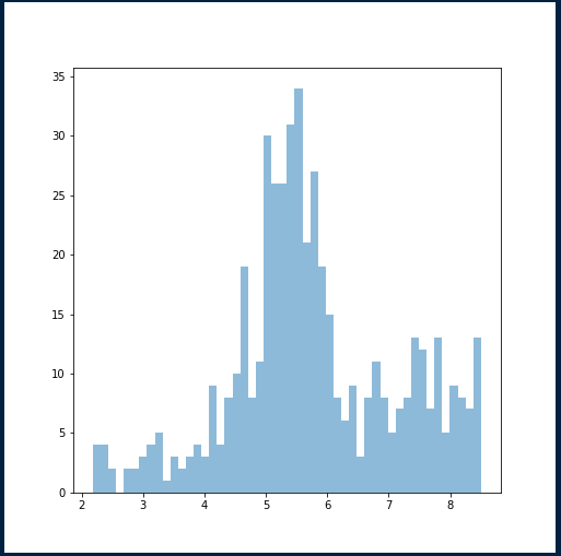
The following plot is just one sample of the training at 5,000 epochs. The more samples you get to iterate the better. Choose one of the samples that approximates close to the original distribution of the data source. We will run a loop for generating ten samples of synthetic data and plot the distributions of all of them as well.

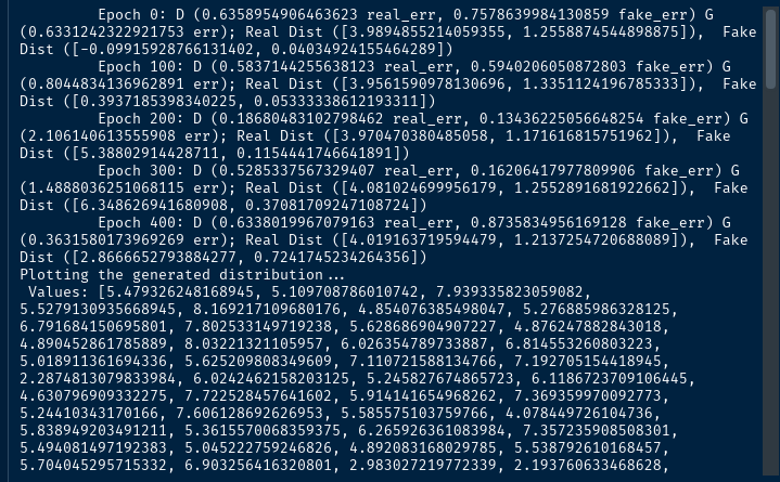
This is the output of each epoch showing some evaluation metrics of the GAN. What we show are:
- The errors in the Discriminator (D) for the real data and the fake data
- The error in the Generator (G)
- The mean and standard deviation for the real data
- The mean and standard deviation for the synthetic data
GAN in rTorch
The following code is the converted code from PyTorch to rTorch. They will look essentially the same. It will be completely up to you if you want to run the PyTorch code in its native Python, or the R version of it. In my particular case I find myself more comfortable working with the R data structures like dataframes, lists and vectors.
This code is almost a literal conversion of the Python code we just have shown above. This code can be found as the file “gan_torch.R” under the folder notebooks.
library(rTorch)

nn       <- torch$nn
optim    <- torch$optim
Variable <- torch$autograd$Variable


# Data params
data_mean <- 4
data_stddev <- 1.25


# lambda functions
name         <- "Only 4 moments"
preprocess   <- function(data) get_moments(data)
d_input_func <- function(x) 4L


get_distribution_sampler <- function(mu, sigma) {
    # torch.Tensor(np.random.normal(mu, sigma, (1, n)))
    # the last member of the normal is the shape vector
    function(n) torch$Tensor(np$random$normal(mu, sigma, c(1L, n)))
}

get_generator_input_sampler <- function(){
    # lambda m, n: torch.rand(m, n)
    function(m, n) torch$rand(m, n)
}

d_sampler <- get_distribution_sampler(data_mean, data_stddev)

get_moments <- function(d) {
    mean <- torch$mean(d)
    diffs <- d - mean
    var <- torch$mean(torch$pow(diffs, 2.0))
    std <- torch$pow(var, 0.5)
    zscores <- diffs / std
    skews <- torch$mean(torch$pow(zscores, 3.0))
    kurtoses <- torch$mean(torch$pow(zscores, 4.0)) - 3.0
    # torch.cat((mean.reshape(1,), std.reshape(1,), skews.reshape(1,), kurtoses.reshape(1,)))
    final <- torch$cat(c(torch$reshape(mean, list(1L)), torch$reshape(std, list(1L)),
                       torch$reshape(skews, list(1L)), torch$reshape(kurtoses, list(1L))))
    return(final)
}


py_run_string("import torch")
main = py_run_string(
"
import torch.nn as nn

class Generator(nn.Module):
    # Two hidden layers
    # Three linear maps
    def __init__(self, input_size, hidden_size, output_size, f):
        super(Generator, self).__init__()
        self.map1 = nn.Linear(input_size, hidden_size)
        self.map2 = nn.Linear(hidden_size, hidden_size)
        self.map3 = nn.Linear(hidden_size, output_size)
        self.f = f

    def forward(self, x):
        x = self.map1(x)
        x = self.f(x)
        x = self.map2(x)
        x = self.f(x)
        x = self.map3(x)
        return x


class Discriminator(nn.Module):
    # also two hidden layer and three linear maps
    def __init__(self, input_size, hidden_size, output_size, f):
        super(Discriminator, self).__init__()
        self.map1 = nn.Linear(input_size, hidden_size)
        self.map2 = nn.Linear(hidden_size, hidden_size)
        self.map3 = nn.Linear(hidden_size, output_size)
        self.f = f

    def forward(self, x):
        x = self.f(self.map1(x))
        x = self.f(self.map2(x))
        return self.f(self.map3(x))
"
)

Generator     <- main$Generator
Discriminator <- main$Discriminator

extract <- function(v){
    return(v$data$storage()$tolist())
}


stats <- function(d) {
    return(list(np$mean(d), np$std(d)))
}

# for 1D list
list_for_cat <- function(li) {
    cum <- ""
    len <- length(li)
    for (i in seq(length(li))) {
        sep <- ifelse(i != len, ", ",  "")
        cum <- paste0(cum, paste0(li[i], sep))
    }
    paste0("[", cum, "]")
}

```


```{r}
train <- function(){
    # Model parameters
    g_input_size <- 1L      # Random noise dimension coming into generator, per output vector
    g_hidden_size <- 5L     # Generator complexity
    g_output_size <- 1L     # Size of generated output vector
    d_input_size <- 500L    # Minibatch size - cardinality of distributions
    d_hidden_size <- 10L    # Discriminator complexity
    d_output_size <- 1L     # Single dimension for 'real' vs. 'fake' classification
    minibatch_size = d_input_size

    d_learning_rate <- 1e-3
    g_learning_rate <- 1e-3
    sgd_momentum <- 0.9

    num_epochs <- 500
    print_interval <- 100
    d_steps <- 20
    g_steps <- 20

    dfe <- 0; dre <- 0; ge <- 0
    d_real_data <- NULL; d_fake_data <- NULL; g_fake_data <- NULL

    # Activation functions
    discriminator_activation_function = torch$sigmoid
    generator_activation_function     = torch$tanh

    d_sampler = get_distribution_sampler(data_mean, data_stddev)
    gi_sampler = get_generator_input_sampler()


    G = Generator(input_size=g_input_size,
                      hidden_size=g_hidden_size,
                      output_size=g_output_size,
                      f=generator_activation_function)

    D = Discriminator(input_size=d_input_func(d_input_size),
                          hidden_size=d_hidden_size,
                          output_size=d_output_size,
                          f=discriminator_activation_function)

    criterion <- nn$BCELoss()  # Binary cross entropy: http://pytorch.org/docs/nn.html#bceloss
    d_optimizer = optim$SGD(D$parameters(), lr = d_learning_rate, momentum = sgd_momentum)
    g_optimizer = optim$SGD(G$parameters(), lr = g_learning_rate, momentum = sgd_momentum)


    # Now, training loop alternates between Generator and Discriminator modes

    for (epoch in (0:num_epochs)) {
        ## cat(sprintf("%5d:", epoch))
        for (d_index in (0:d_steps)) {
            ## cat(sprintf("%3d", d_index))

            # 1. Train D on real+fake
            D$zero_grad()

            #  1A: Train D on real data
            d_real_data = Variable(d_sampler(d_input_size))
            d_real_decision = D(preprocess(d_real_data))
            d_real_error = criterion(d_real_decision, Variable(torch$ones( list(1L, 1L) )))  # ones = true
            d_real_error$backward()  # compute/store gradients, but don't change params

            #  1B: Train D on fake data
            d_gen_input = Variable(gi_sampler(minibatch_size, g_input_size))
            d_fake_data = G(d_gen_input)$detach()  # detach to avoid training G on these labels
            d_fake_decision = D(preprocess(d_fake_data$t()))
            d_fake_error = criterion(d_fake_decision, Variable(torch$zeros( list(1L, 1L) )))  # zeros = fake
            d_fake_error$backward()
            # Only optimizes D's parameters; changes based on stored gradients from backward()
            d_optimizer$step()

            dre <- extract(d_real_error)[1]; dfe <- extract(d_fake_error)[1]

        }
        ## cat("\n")

        for (g_index in (1:g_steps)){
                # 2. Train G on D's response (but DO NOT train D on these labels)
                G$zero_grad()

                gen_input = Variable(gi_sampler(minibatch_size, g_input_size))
                g_fake_data = G(gen_input)
                dg_fake_decision = D(preprocess(g_fake_data$t()))
                # Train G to pretend it's genuine
                g_error = criterion(dg_fake_decision, Variable(torch$ones( list(1L, 1L) )))

                g_error$backward()
                g_optimizer$step()  # Only optimizes G's parameters
                ge = extract(g_error)[1]
        }

        if ((epoch %% print_interval) == 0) {
            cat(sprintf("\t Epoch %4d: D (%8f5 real_err, %8f5 fake_err) G (%8f5 err); Real Dist (%s),  Fake Dist (%s) \n",
                        epoch, dre, dfe, ge,
                        list_for_cat(stats(extract(d_real_data))),
                        list_for_cat(stats(extract(d_fake_data))) ))
        }
    }
    print("Plotting the generated distribution...")
    values = extract(g_fake_data)
    cat(sprintf(" Values: %s", str(values)))
    hist(values, breaks = 50, col =  "lightblue")
}

train()
This is is the output data from R.
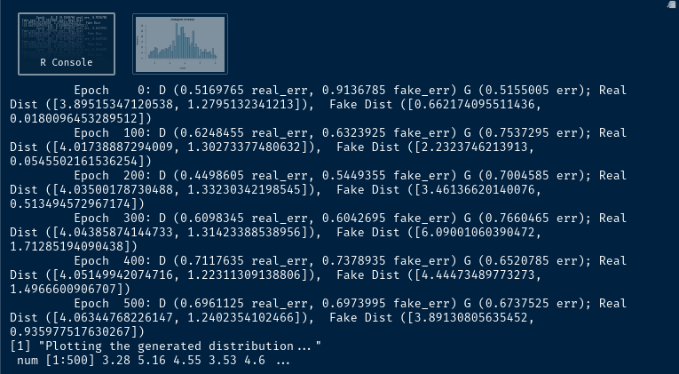
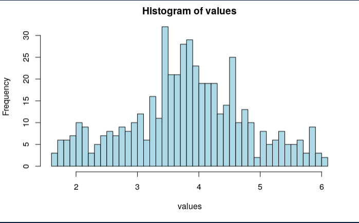
And this is the histogram in R. No fancy things here; just plain, simple r-base. This is the result of running the training for 5,000 epochs.
Motivation
For the moment, I just wanted to share the preliminary results of the converted code. Both versions, in Python and R, run fine. I have managed to generate additional runs on the train() function to find out how the fake data (synthetic) distribution behaves, or how different is from the real data. My second objective is to show the differences in coding in PyTorch vs rTorch. They are pretty similar with exception of the obvious language differences and the way we pass parameters to the PyTorch library. For instance, an integer has to be explicitly declared in R when calling a PyTorch function (0L, 1L, 2L). Or, when you need to pass a tuple for the shape of a tensor, you should use c() or list() in R. But it mostly fun. Additionally, I wanted to test my rTorch package with a real application such as this GAN.
Findings
- Each run of 5,000 epochs takes approximately 20 minutes, without a GPU.
- You can try reducing the number of epochs in the training to, let’s say, 500. I invite you to do it and see the shape of the distribution for the synthetic data. It won’t be the same quality as the distribution at 5,000 epochs.
- When I say quality, I mean how much the synthetic data resembles the real or original data. We use the mean and standard deviation as part of the evaluation metrics.
- Plotting the synthetic data histogram is also a good guidance of how well it approximates to the real data.
Code
The code has been published in GitHub (Python and R). I used R, RStudio, Python Anaconda3 for 64-bits, and the R packages reticulate, rTorch, rsuite, ggplot2. On the Python side, PyTorch, numpy, pandas, matplotlib. I tried to avoid using matplotlib and use ggplot2 instead.
In the next episodes of these series, I will publish a real petroleum engineering dataset converted to synthetic data, so you could feel the difference. I was thinking on the Volve reservoir simulation data which already has been published.
There are lots to be learned by comparing a synthetic dataset versus the original dataset, starting with a simple Exploratory Data Analysis (EDA).
In the next episode
- Plot of the real data distribution
- Plots of 10 sets of synthetic data at 500 epochs and 5,000 epochs
- How do we know we obtained a good set of synthetic data
Code
References
- Original article “Generative Adversarial Networks (GANs) in 50 lines of code (PyTorch)" by Dev Nag. This is the article that made get hooked in GANs.
- Paper “Privacy and Synthetic Datasets”, by Steven M. Bellovin, Preetam K. Dutta, and Nathan Reitinger. 2019.
- Article “An introduction to Generative Adversarial in TensorFlow” by John Glover. 2019.
- Paper “Generative Adversarial Nets” by Goodfellow, Pouget-Abadie, Mirza, Xu, Warde-Farley, Ozair, Courville and Bengio. 2014.
- Paper “[Improved Techniques for Training GANs](http://Improved Techniques for Training GANs)”, by Tim Salimans, Ian Goodfellow, Wojciech Zaremba, Alec Radford, Vicki Cheung, Xi Chen. 2016.
- Article “Artificial data give the same results as real data — without compromising privacy” by Stefanie Koperniak. 2017.
- Article “Synthetic data, privacy, and the law” by Brad Wible. Science 2019.