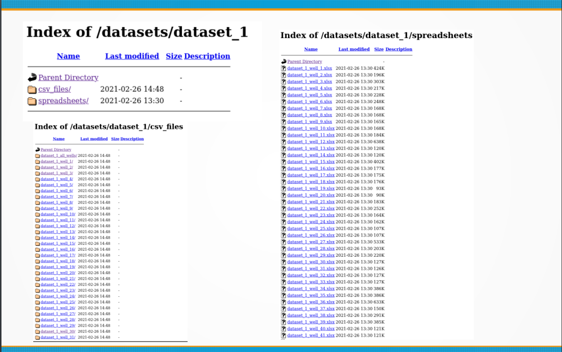
Okay. There are two ways of downloading the data for all the wells in the SPE repository: the manual way (one file at a time with “Save As”), and the non-interactive automated way. The manual way is the easiest and require that you provide your SPE username and password in your usual login page. Then, you click on the link to the repository https://www.spe.org/datasets/, and start right-clicking on each of the files under the data folders. Then select the menu option “Save As” on each of the file links. The only drawback of doing it this way is that will have to do it 53 x 3 times, because there are 53 well folders and three files per folder.
For the CSV files, this is the list of folders. It will go like this until well_53:
Read the first well in non-interactive model
If you want to do this in non-interactive mode, you will need to supply your SPE user name and password from a script, to authorize access to the machine, and then the script will automatically download the files. There are many ways to do it. As an example, for one well, well_1, in CSV format with R using the package rvest, the commands would be:
library(rvest)
url <- "https://spe.org/en/login/"
pgsession <- html_session(url)
pgform <- html_form(pgsession)[[1]]
filled_form <- set_values(pgform,
"se_Username" = "first.last@example.com",
"s_Password" = "my_secret")
submit_form(pgsession,filled_form)
dataset_url <- "https://www.spe.org/datasets/dataset_1/csv_files/dataset_1_well_1/deviation_survey"
raw_page <- jump_to(pgsession, dataset_url)
page_html <- xml2::read_html(raw_page$response)
page_text <- html_text(page_html)
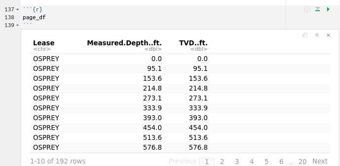
page_df <- read.table(text = page_text, header = TRUE, sep = ",")
print(dim(page_df))
Which output would be:
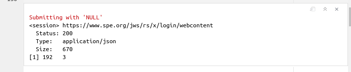
This means that well_1 has 192 observations (rows) and 3 features or variables (columns).
If we want to take a quick look at the data structure:
Explanation
The first two functions html_session() and html_form() provide us the form for the login page at https://spe.org/en/login. With the set_values() function we provide the user name, which is really your email address you use to login to SPE, and the password. se_Username and s_Password are the identifiers for those two inputs in the HTML form. After logging in, we supply the page link with the desired dataset with the function jump_to(). For the well_1 case, the dataset_url will be
"https://www.spe.org/datasets/dataset_1/csv_files/dataset_1_well_1/deviation_survey"
Then we read the html raw data of the response with read_html() , convert it to text with html_text(). The last step is converting the text string in page_text with the function read.table(), to finally obtain the dataframe with the well survey data.
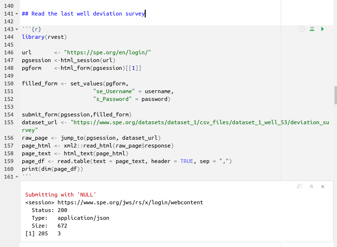
Read the last well in non-interactive mode
The last CSV well files are located under the folder dataset_1_well_53. To read that well we use a similar strategy to the first well. The only difference that you will notice in this script is the name of the dataset, and that now we are providing two objects: username and password. You could do the same if you assign your SPE user name and password to two R objects or variables outside the script so you don’t share your private data accidentally.
Read deviation_survey from dataset_1_all_wells
The dataset_1_all_wells folder is located under this URL https://www.spe.org/datasets/dataset_1/csv_files/dataset_1_all_wells/. There are three files in there: the deviation_survey, production_data, and the well_data. Pretty similar to what we did for the first and last well, but now we change the dataset URL to:
"https://www.spe.org/datasets/dataset_1/csv_files/dataset_1_all_wells/deviation_survey"
The code for that operation is:
library(rvest)
url <- "https://spe.org/en/login/"
pgsession <-html_session(url)
pgform <-html_form(pgsession)[[1]]
filled_form <- set_values(pgform,
"se_Username" = username,
"s_Password" = password)
submit_form(pgsession,filled_form)
all_datasets_url <- "https://www.spe.org/datasets/dataset_1/csv_files/dataset_1_all_wells/deviation_survey"
all_raw_page <- jump_to(pgsession, all_datasets_url)
all_page_html <- xml2::read_html(all_raw_page$response)
all_page_text <- html_text(all_page_html)
all_page_df <- read.table(text = all_page_text, header = TRUE, sep = ",")
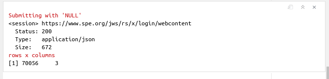
message("rows x columns")
print(dim(all_page_df))
which gives us a total of 70056 rows or observations!
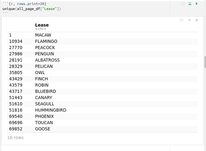
If we want to know the number of leases in that dataset we use the function unique():
Read the rest all of the well deviation surveys
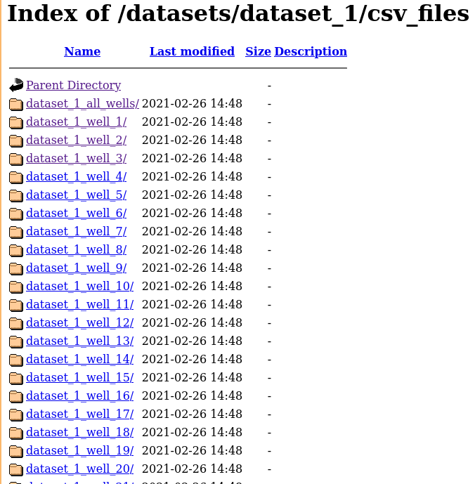
If you take a look at the well folder for CSV files, you will find 53 wells:
	dataset_1_well_1/	2021-02-26 14:48	-
	dataset_1_well_2/	2021-02-26 14:48	-
	dataset_1_well_3/	2021-02-26 14:48	-
	dataset_1_well_4/	2021-02-26 14:48	-
	dataset_1_well_5/	2021-02-26 14:48	-
	dataset_1_well_6/	2021-02-26 14:48	-
	dataset_1_well_7/	2021-02-26 14:48	-
	dataset_1_well_8/	2021-02-26 14:48	-
	dataset_1_well_9/	2021-02-26 14:48	-
	dataset_1_well_10/	2021-02-26 14:48	-
	dataset_1_well_11/	2021-02-26 14:48	-
	dataset_1_well_12/	2021-02-26 14:48	-
	dataset_1_well_13/	2021-02-26 14:48	-
	dataset_1_well_14/	2021-02-26 14:48	-
	dataset_1_well_15/	2021-02-26 14:48	-
	dataset_1_well_16/	2021-02-26 14:48	-
	dataset_1_well_17/	2021-02-26 14:48	-
	dataset_1_well_18/	2021-02-26 14:48	-
	dataset_1_well_19/	2021-02-26 14:48	-
	dataset_1_well_20/	2021-02-26 14:48	-
	dataset_1_well_21/	2021-02-26 14:48	-
	dataset_1_well_22/	2021-02-26 14:48	-
	dataset_1_well_23/	2021-02-26 14:48	-
	dataset_1_well_24/	2021-02-26 14:48	-
	dataset_1_well_25/	2021-02-26 14:48	-
	dataset_1_well_26/	2021-02-26 14:48	-
	dataset_1_well_27/	2021-02-26 14:48	-
	dataset_1_well_28/	2021-02-26 14:48	-
	dataset_1_well_29/	2021-02-26 14:48	-
	dataset_1_well_30/	2021-02-26 14:48	-
	dataset_1_well_31/	2021-02-26 14:48	-
	dataset_1_well_32/	2021-02-26 14:48	-
	dataset_1_well_33/	2021-02-26 14:48	-
	dataset_1_well_34/	2021-02-26 14:48	-
	dataset_1_well_35/	2021-02-26 14:48	-
	dataset_1_well_36/	2021-02-26 14:48	-
	dataset_1_well_37/	2021-02-26 14:48	-
	dataset_1_well_38/	2021-02-26 14:48	-
	dataset_1_well_39/	2021-02-26 14:48	-
	dataset_1_well_40/	2021-02-26 14:48	-
	dataset_1_well_41/	2021-02-26 14:48	-
	dataset_1_well_42/	2021-02-26 14:48	-
	dataset_1_well_43/	2021-02-26 14:48	-
	dataset_1_well_44/	2021-02-26 14:48	-
	dataset_1_well_45/	2021-02-26 14:48	-
	dataset_1_well_46/	2021-02-26 14:48	-
	dataset_1_well_47/	2021-02-26 14:48	-
	dataset_1_well_48/	2021-02-26 14:48	-
	dataset_1_well_49/	2021-02-26 14:48	-
	dataset_1_well_50/	2021-02-26 14:48	-
	dataset_1_well_51/	2021-02-26 14:48	-
	dataset_1_well_52/	2021-02-26 14:48	-
	dataset_1_well_53/	2021-02-26 14:48	-
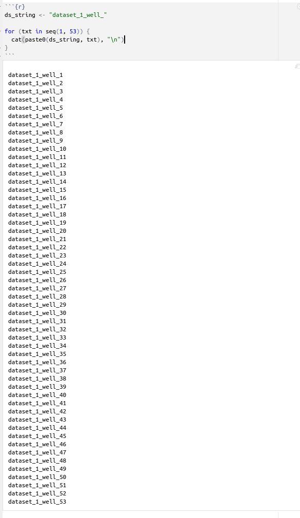
Each of these folders contain three files: deviation survey, production data, and generic well data. We will collect now the deviation survey for each of these wells by changing the well identifier from 1 to 53. The URL for that well is associated with the well number. To make this a variable string, we use a for-loop together with the concatenation function paste0(), of a well string plus the well id which is provided by the function seq(1, 53). Like this:
ds_string <- "dataset_1_well_"


for (txt in seq(1, 53)) {
  cat(paste0(ds_string, txt), "\n")
}
You get the idea.
Once you execute it, it will be giving you the output you are looking for (see below)
Then we integrate this for-loop into one of the code chunks we were using for the first or the last well. The code would look like this:
library(rvest)


url       <- "https://spe.org/en/login/"
pgsession <-html_session(url)


pgform    <-html_form(pgsession)[[1]]


filled_form <- set_values(pgform,
                      "se_Username" = username,
                      "s_Password" = password)


submit_form(pgsession,filled_form)


ds_string <- "dataset_1_well_"
df <- data.frame()
for (txt in seq(1, 53)) {
  well_x_url <- paste0("https://www.spe.org/datasets/dataset_1/csv_files/",
                       ds_string, txt, "/deviation_survey")
  cat(well_x_url, "\n")
  well_x_raw_page <- jump_to(pgsession, well_x_url)
  well_x_page_html <- xml2::read_html(well_x_raw_page$response)
  well_x_page_text <- html_text(well_x_page_html)
  well_x_df <- read.table(text = well_x_page_text, header = TRUE, sep = ",")
  df <- rbind(df, well_x_df)
}
with the following output:
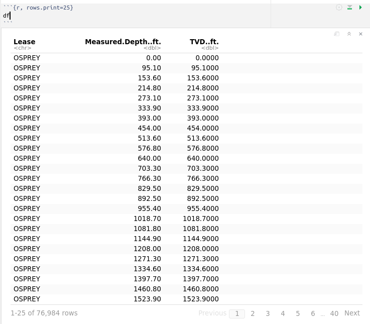
There are 76,984 rows or observations.
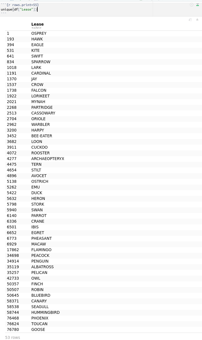
Let’s see how many unique leases we got for this command:
unique(df["Lease"])
Confusion and comparison
By this time you are wondering why we are collecting the data from individual data if we have already a dataset called dataset_1_all_wells. Wasn’t this dataset supposed to contain all the well data?
We don’t know yet. Some wells from the individual collection may be contained in this dataset_1_all_wells dataset. We have to be sure. The next step is finding if any of the individual well data is already repeating. So, what we have to do is comparing subsets of data, and if they are repeated, set it aside and explain.
How do we do that?
First, we will plot MD vs TVD for the wells in the dataset dataset_1_all_wells. And then we’ll do a quick comparison of the deviation surveys against the ones we obtained from the for-loop collection we called df.
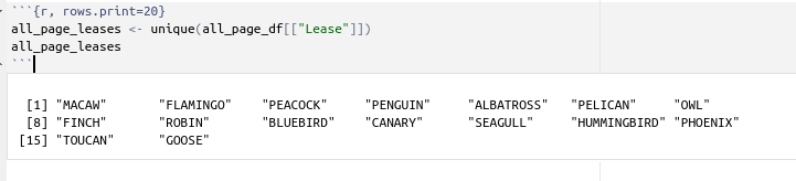
But first we get the list of all the leases in dataset_1_all_wells.
all_page_leases <- unique(all_page_df[["Lease"]])
all_page_leases
which gives us sixteen leases:
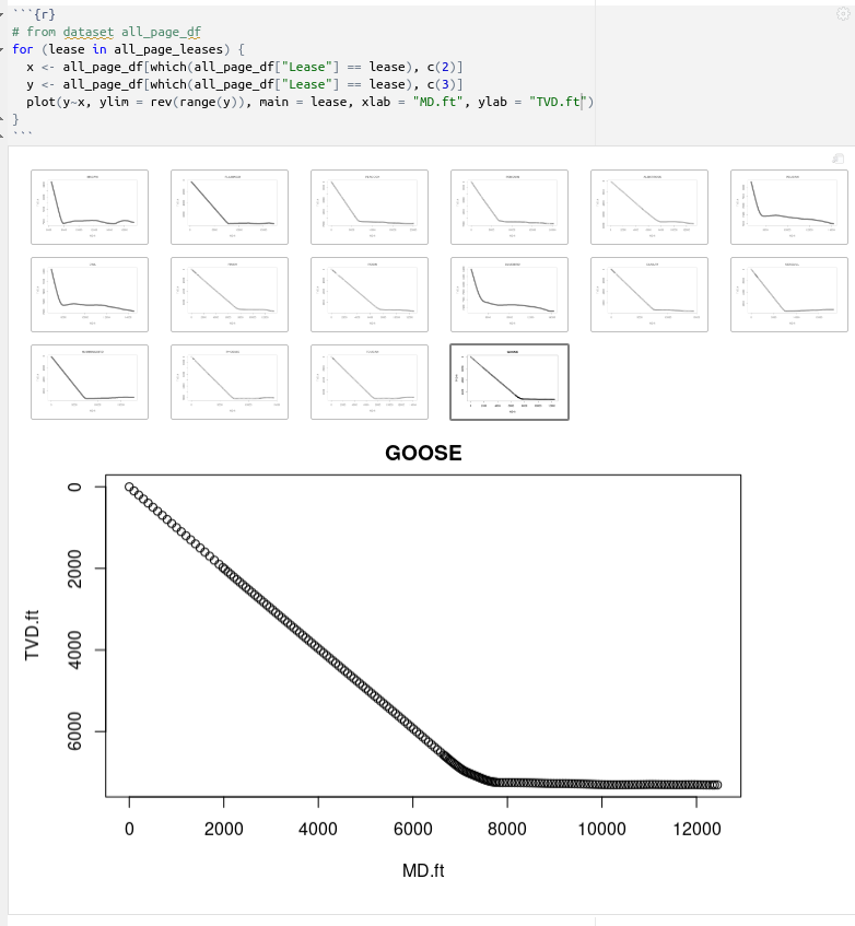
Plot deviation surveys in dataset dataset_1_all_wells
We use a for-loop to iterate through all the leases we want them plotted:
# from dataset all_page_df
for (lease in all_page_leases) {
  x <- all_page_df[which(all_page_df["Lease"] == lease), c(2)]
  y <- all_page_df[which(all_page_df["Lease"] == lease), c(3)]
  plot(y~x, ylim = rev(range(y)), main = lease)
}
which gives us:
Plot deviation surveys in the for-loop collected dataset *df*
# from dataset all_page_df
for (lease in all_page_leases) {
  # plot(all_page_df[which(all_page_df["Lease"] == lease), c(2,3)] )
  x <- all_page_df[which(all_page_df["Lease"] == lease), c(2)]
  y <- all_page_df[which(all_page_df["Lease"] == lease), c(3)]
  plot(y~x, ylim = rev(range(y)), main = lease, xlab = "MD.ft", ylab = "TVD.ft")
}
which gives us all these plots:
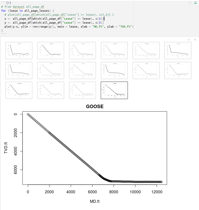
If you a quick visual comparison, you will see that we have repeating data. We should prefer working with the collected dataset we obtained with the for-loop.
NOTE. I am omitting the use of the R packages dplyr and ggplot2 on purpose. For the best learning experience of R, it is better to get familiarized first with base R.
Comparing seemingly equal datasets the right way
That was the quick visual comparison. At first sight both deviation surveys from the all_wells dataset and the merged_wells dataset seem the same. But how can we be 100% sure? There are many ways two deviation survey could appear similar but still be different:
- They start at different depths but the number of points is the same
- They finish at different depths but the number of points is the same
- The spacing between points may change but the number of points is still the same
- The number of points is still the same but they are in different units (feet vs meters)
So, we need to be sure that they are identically similar before moving on. The MDs from one dataset must the equal to the MDs of the second, merged, dataset. We can do this by comparing the counts and then comparing the MD and TVD vectors value by value.
Compare the counts or number of points in the deviation survey
Here what we do is simply compare the counts or number of points that each deviation survey contains; the one coming from the dataset all_wells versus the data coming from the merged_wells dataset. We do that by using the function length(x1)==length(x2). x1 corresponds to the MD of all_wells, x2 contains the MD values from merged_wells. y1 and y2 correspond to TVDs.
# get number of leases from all_wells dataset
all_wells_devsurv <- all_page_df    # copy dataframe to more meaningful object name
all_wells_devsurv_leases <- unique(all_wells_devsurv[["Lease"]])
sort(all_wells_devsurv_leases)


# iterate through leases of interest and compare number of observations
cat(sprintf("%12s %9s %9s %10s %9s %9s %10s", "Lease", "MD.ft", "MD.ft", "count_eq",
             "TVD.ft", "TVD.ft", "count_eq"), "\n")
cat(sprintf("%22s %9s %20s %9s", "all_wells", "merged", "all_wells", "merged"), "\n")
for (lease in all_wells_devsurv_leases) {
  # all_wells dataset. extract MD and TVD
  x1 <- all_wells_devsurv[which(all_wells_devsurv["Lease"] == lease), c(2)]
  y1 <- all_wells_devsurv[which(all_wells_devsurv["Lease"] == lease), c(3)]
  # combined/merged dataset.extract MD and TVD
  x2 <- merged_wells_devsurvey[which(merged_wells_devsurvey["Lease"] == lease), c(2)]
  y2 <- merged_wells_devsurvey[which(merged_wells_devsurvey["Lease"] == lease), c(3)]
  cat(sprintf("%12s %9d %9d %10s %9d %9d %10s \n", lease, length(x1), length(x2),
              length(x1) == length(x2),
              length(y1), length(y2),
              length(y1) == length(y2)
              ))
}
which will yield the following output:
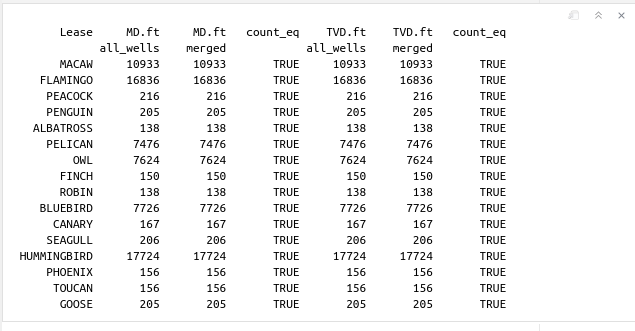
Again, comparing the counts is not enough to conclude that MD, TVD from both datasets are identical. We need to do something else.
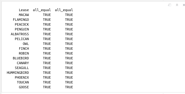
Compare values at every point of the deviation survey
Here we compare the MD and TVD vectors of each well with a logical equality such as x1==x2, where x1 is a vector with all MD measurements from the all_wells dataset, and x2 is a vector with the MD values for the deviation survey in the merged_wells dataset. Notice the use of the function all(x1==x2). If we print x1==x2, and let’s say, the deviation survey for that well has 10,000 points, then we would get 10,000 TRUE values. We don’t need to print all the values that are all equal. The function all() is equivalent of the boolean operator AND. So, if all the 10,000 MD and TVD comparisons are TRUE, the result of AND(TRUE, TRUE, TRUE, …) will be only one value: TRUE. And that should be enough.
# iterate through leases of interest
cat(sprintf("%12s %10s %10s \n", "Lease", "all_equal", "all_equal"))
for (lease in all_wells_devsurv_leases) {
  # all_wells dataset. MD, TVD
  x1 <- all_wells_devsurv[which(all_wells_devsurv["Lease"] == lease), c(2)]
  y1 <- all_wells_devsurv[which(all_wells_devsurv["Lease"] == lease), c(3)]
  # merged dataset MD, TVD
  x2 <- merged_wells_devsurvey[which(merged_wells_devsurvey["Lease"] == lease), c(2)]
  y2 <- merged_wells_devsurvey[which(merged_wells_devsurvey["Lease"] == lease), c(3)]
  cat(sprintf("%12s %10s %10s \n", lease,
              all(x1 == x2),
              all(y1 == y2)
              ))
}
This is the output: